
Differences in Means: Surveys and Experiments
Our survey design and estimator
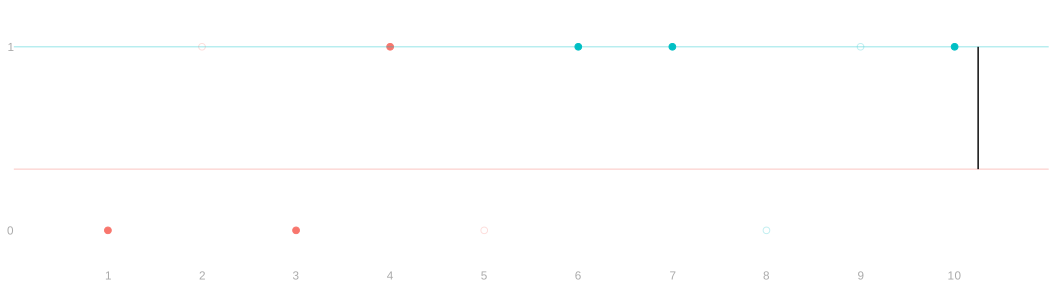
We will use stratified sampling:
- we fix how many to sample from each subpopulation,
- then sample within each one separately, without replacement.
We take numbered cards within our own subpopulation,
- shuffle a deck for each, and take the top three.
The difference in sample means is our estimator:
\hat\Delta=\textcolor{#00BFC4}{\hat\mu(1)}-\textcolor{#F8766D}{\hat\mu(0)}.
Interval estimation
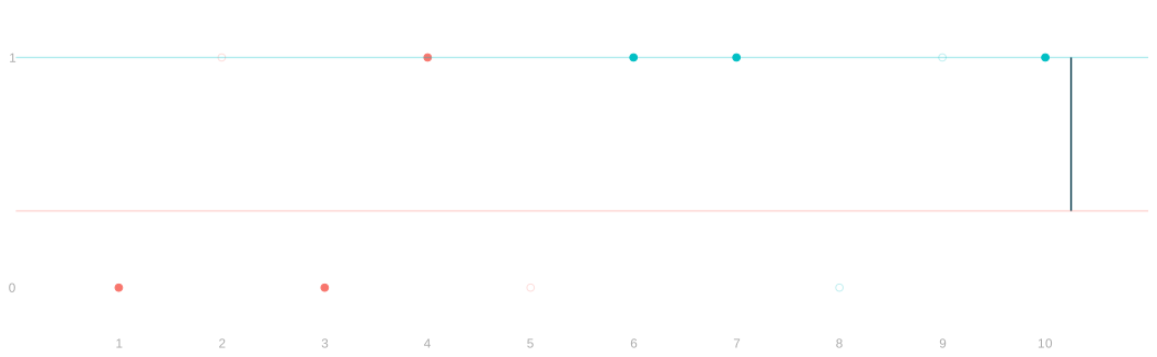
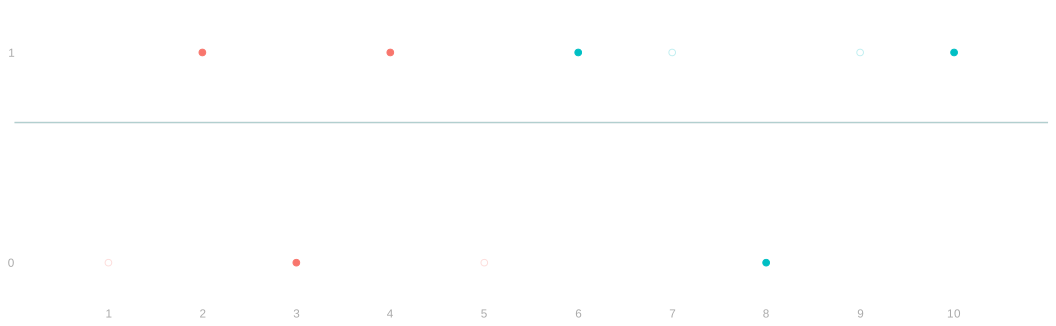
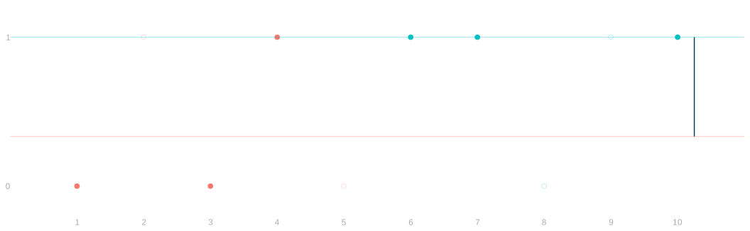
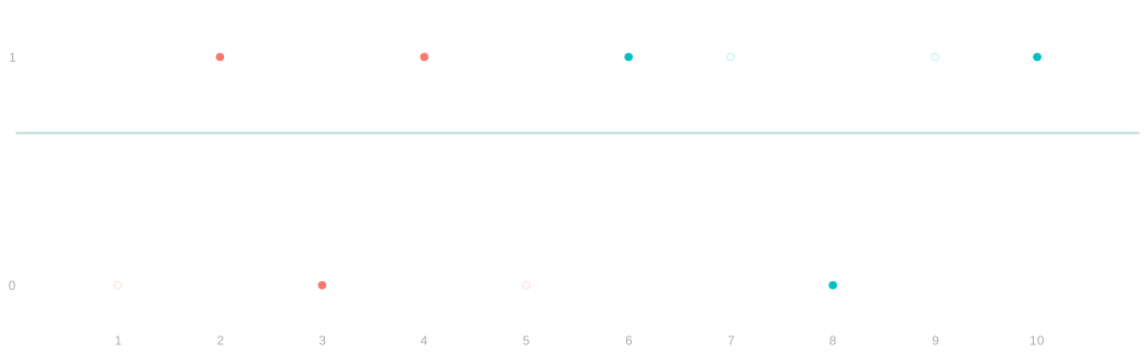
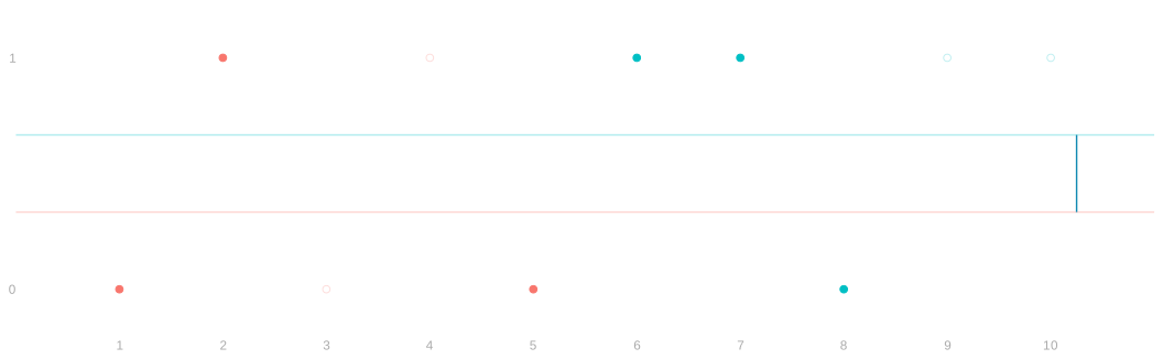
- That gives a point estimate. How do we get an interval estimate?
- An interval estimate depends on the sampling distribution of \hat\Delta.
- We will have to collect responses from everybody else.
- With the whole population written down, we can rerun the survey from it:
- shuffle the two decks again, take three more from each subpopulation,
- and get another estimate.
- What do we see?
Unbiasedness
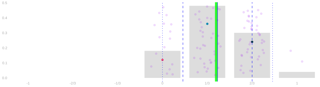
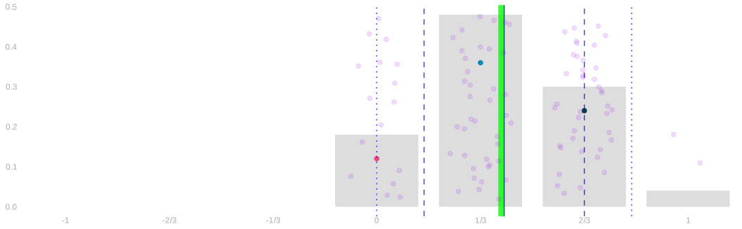
- The sampling distribution is centered on \Delta. How did we know?
- From the two subpopulations separately:
- each sample mean is unbiased for its own subpopulation’s mean,
- and an expectation of a difference is the difference of expectations.
Could we calculate the width?
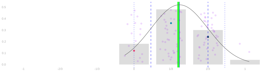
- What is the variance of our estimate?
The two samples are drawn independently, so
\operatorname{Var}(\hat\Delta)=\operatorname{Var}\{\textcolor{#00BFC4}{\hat\mu(1)}\}+\operatorname{Var}\{\textcolor{#F8766D}{\hat\mu(0)}\}, \qquad \operatorname{Var}\{\hat\mu(w)\}=\frac{\sigma^2(w)}{n_w}\frac{m_w-n_w}{m_w-1}.
What does this tell us about choosing our sample sizes?
- Enlarging one sample leaves the other subpopulation’s term alone.
- However many we sample from one, a small sample in the other still limits our precision.
- The gray curve is the normal approximation with that variance.
- At three per subpopulation it is poor.
How can we estimate this distribution more precisely?

| p | \textcolor{#F8766D}{\hat\mu(0)} | \textcolor{#00BFC4}{\hat\mu(1)} | \hat\Delta |
|---|---|---|---|
| \textcolor{#073B4C}{\frac{3}{10}\cdot\frac{3}{5}=\frac{9}{50}} | \textcolor{#F8766D}{2/3} | \textcolor{#00BFC4}{2/3} | \textcolor{#073B4C}{0} |
| \textcolor{#EF476F}{\frac{6}{10}\cdot\frac{3}{5}=\frac{18}{50}} | \textcolor{#F8766D}{1/3} | \textcolor{#00BFC4}{2/3} | \textcolor{#EF476F}{1/3} |
| \textcolor{#EF476F}{\frac{3}{10}\cdot\frac{2}{5}=\frac{6}{50}} | \textcolor{#F8766D}{2/3} | \textcolor{#00BFC4}{1} | \textcolor{#EF476F}{1/3} |
| \textcolor{#118AB2}{\frac{1}{10}\cdot\frac{3}{5}=\frac{3}{50}} | \textcolor{#F8766D}{0} | \textcolor{#00BFC4}{2/3} | \textcolor{#118AB2}{2/3} |
| \textcolor{#118AB2}{\frac{6}{10}\cdot\frac{2}{5}=\frac{12}{50}} | \textcolor{#F8766D}{1/3} | \textcolor{#00BFC4}{1} | \textcolor{#118AB2}{2/3} |
| \textcolor{#06D6A0}{\frac{1}{10}\cdot\frac{2}{5}=\frac{2}{50}} | \textcolor{#F8766D}{0} | \textcolor{#00BFC4}{1} | \textcolor{#06D6A0}{1} |
We sample the subpopulations separately,
- so each row’s probability p is the product of its two sample-mean probabilities.
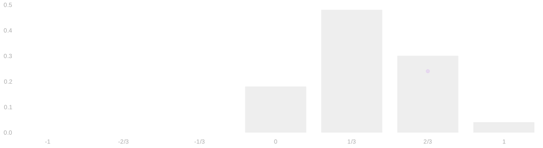
Adding the rows that share a difference gives the distribution exactly:
P(\hat\Delta=d)=\sum_{\textcolor{#00BFC4}{\hat\mu(1)}-\textcolor{#F8766D}{\hat\mu(0)} \,=\, d} p.
Can we always use this survey design?
- Why or why not?
- To use stratified sampling, we need to know which subpopulation every person is in, that is w_j, in advance.
- Sometimes we do. Sometimes we need to call the person up to find their subpopulation.
- In the latter case, we’ll need some new math. We’ll do it later.
Our experiment
- We will taste the same two candies.
- The prime is different: coconut milk chocolate.
- One shuffle of the whole class’s cards picks six people to eat it.
- The groups are randomly assigned. That is what an experiment is.
Again our estimate is the difference in the two sample means.
\hat\Delta=\textcolor{#00BFC4}{\hat\mu(1)}-\textcolor{#F8766D}{\hat\mu(0)}.
How do you calibrate a confidence interval? We simulate our study.
Repeating the experiment
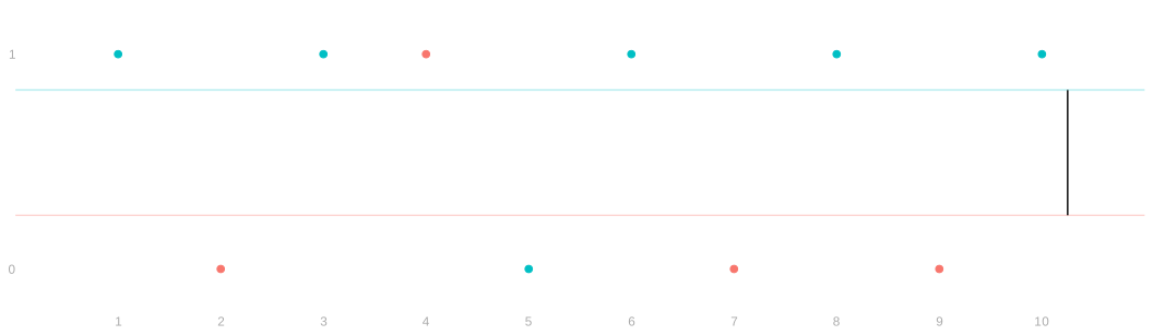
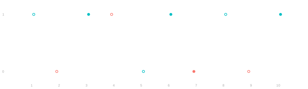
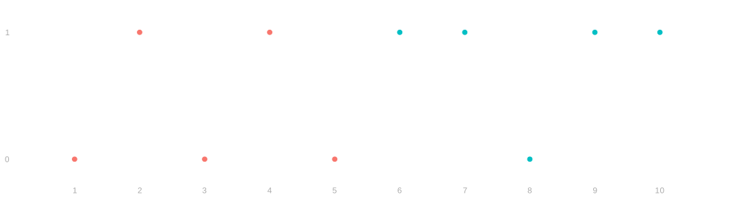
| j | 1 | 2 | 3 | 4 | 5 | 6 | 7 | 8 | 9 | 10 |
|---|---|---|---|---|---|---|---|---|---|---|
| w_j | \color{#00BFC4}1 | \color{#F8766D}0 | \color{#00BFC4}1 | \color{#F8766D}0 | \color{#00BFC4}1 | \color{#00BFC4}1 | \color{#F8766D}0 | \color{#00BFC4}1 | \color{#F8766D}0 | \color{#00BFC4}1 |
| y_j | \color{#00BFC4}1 | \color{#F8766D}0 | \color{#00BFC4}1 | \color{#F8766D}1 | \color{#00BFC4}0 | \color{#00BFC4}1 | \color{#F8766D}0 | \color{#00BFC4}1 | \color{#F8766D}0 | \color{#00BFC4}1 |
As always, we collect the population’s responses and simulate our study.
| j | 1 | 2 | 3 | 4 | 5 | 6 | 7 | 8 | 9 | 10 |
|---|---|---|---|---|---|---|---|---|---|---|
| y_j | ? | ? | \color{#00BFC4}1 | ? | ? | \color{#00BFC4}1 | \color{#F8766D}0 | ? | ? | \color{#00BFC4}1 |
Potential outcomes and treatment effects
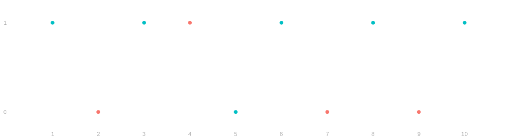
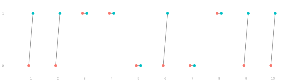
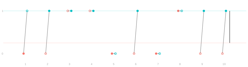
| j | 1 | 2 | 3 | 4 | 5 | 6 | 7 | 8 | 9 | 10 |
|---|---|---|---|---|---|---|---|---|---|---|
| y_j(0) | \color{#F8766D}0 | \color{#F8766D}1 | \color{#F8766D}0 | \color{#F8766D}0 | ||||||
| y_j(1) | \color{#00BFC4}1 | \color{#00BFC4}1 | \color{#00BFC4}0 | \color{#00BFC4}1 | \color{#00BFC4}1 | \color{#00BFC4}1 |
| j | 1 | 2 | 3 | 4 | 5 | 6 | 7 | 8 | 9 | 10 |
|---|---|---|---|---|---|---|---|---|---|---|
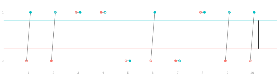
| y_j(0) | 0 | \color{#F8766D}0 | 1 | \color{#F8766D}1 | 0 | 0 | \color{#F8766D}0 | 1 | \color{#F8766D}0 | 0 |
| y_j(1) | \color{#00BFC4}1 | 1 | \color{#00BFC4}1 | 1 | \color{#00BFC4}0 | \color{#00BFC4}1 | 0 | \color{#00BFC4}1 | 1 | \color{#00BFC4}1 |
We say that \textcolor{#F8766D}{y_j(0)} and \textcolor{#00BFC4}{y_j(1)} are person j’s preferences without and with the prime.
We observed y_j(w_j), one of the two. A new assignment asks for the other.
We define the average treatment effect as the mean individual difference:
\Delta=\frac{1}{m}\sum_{j=1}^m \{\textcolor{#00BFC4}{y_j(1)}-\textcolor{#F8766D}{y_j(0)}\}.
- How do we complete it? How do we simulate?
- In this particular context, we can just ask. And then we can run our replication.
- But do you completely buy this?
- How do you really know how eating the chocolate or not ahead of time would have impacted your experience?
- But do you completely buy this?
- How do you really know how eating the chocolate or not ahead of time would have impacted your experience?
- Imagine this was a vaccine.
- If you don’t give someone a vaccine in an experiment and then they get sick,
- you can’t run it again
- and see if the vaccine would have prevented them from getting sick.
- Because they’ve already developed some immunity.
Simulating the experiment
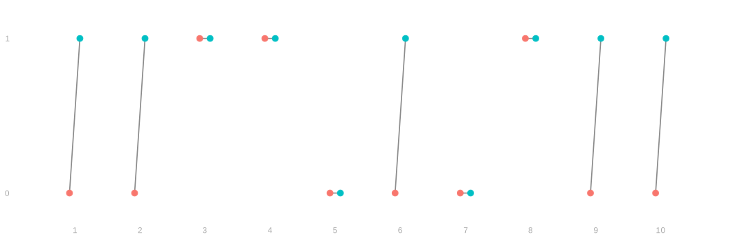
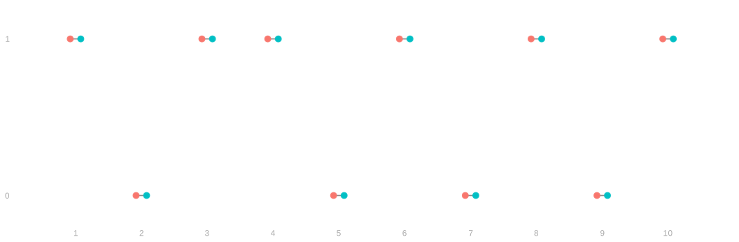
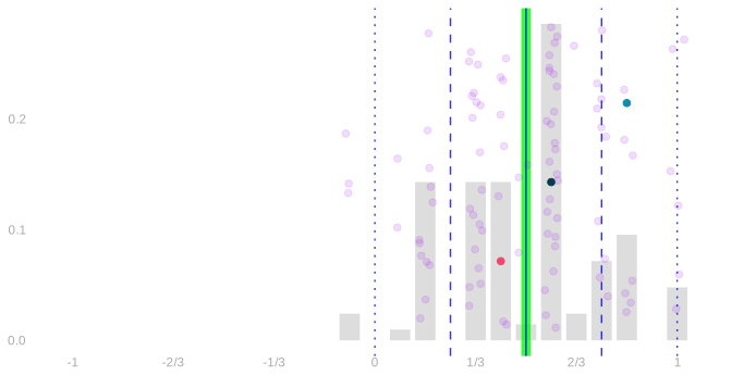
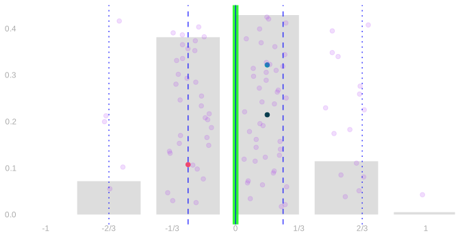
- If you’re going to simulate these things, you need the potential outcome population.
- We can do this a couple times,
- with a couple different ways of filling things in,
- and plot the randomization distributions.
- This is a thing you can do if and only if you know all the potential outcomes,
- which you don’t.
Can we still get an interval estimate?
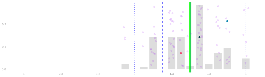
That’s not saying we can’t get an interval estimate.
- That’s just saying we can’t do it by simulating the population we observed in the experiment.
So: can we do this using our observations? Yes and no.
Our estimate is going to stay unbiased.
- Chance decides who is treated, so each group’s mean is unbiased for the corresponding average of potential outcomes:
\begin{aligned} \mathbb E(\hat\Delta)&=\mathbb E\{\textcolor{#00BFC4}{\hat\mu(1)}\}-\mathbb E\{\textcolor{#F8766D}{\hat\mu(0)}\}\\ &=\frac{1}{m}\sum_{j=1}^m \textcolor{#00BFC4}{y_j(1)}-\frac{1}{m}\sum_{j=1}^m \textcolor{#F8766D}{y_j(0)}=\Delta. \end{aligned}
So the question boils down to whether we can do spread.
- The spread does not split into the two groups’ terms as it did in the survey. It depends on both of each person’s potential responses, of which we only ever see one.
A pitfall
- Population A
- Population B
- Population A
- Population B
- Population A
- Population B
- Population A
- Population B
- Population A
- Population B
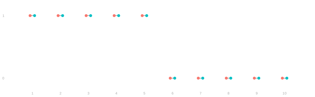
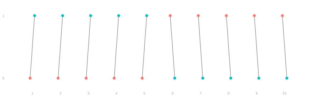
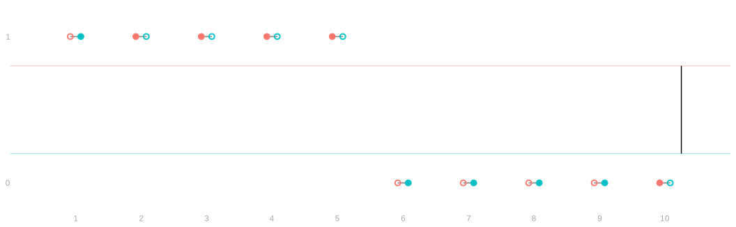
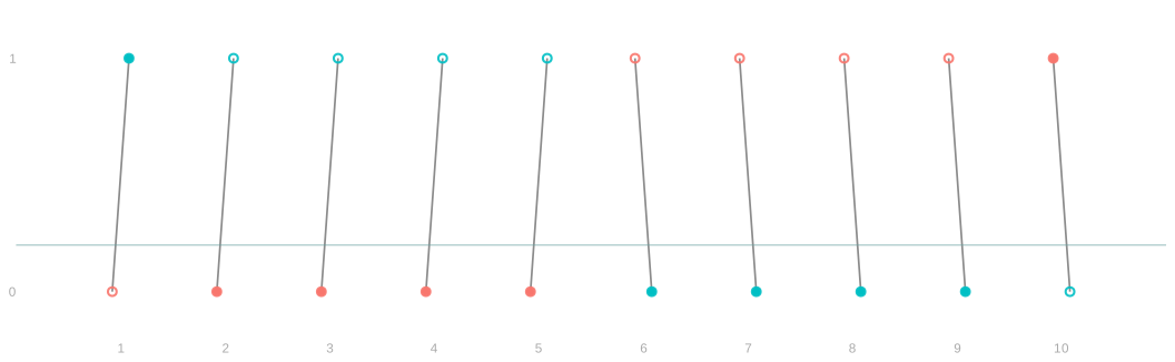
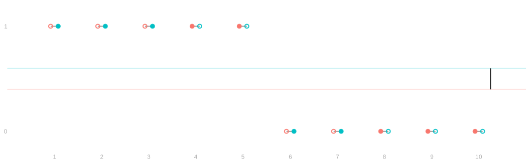
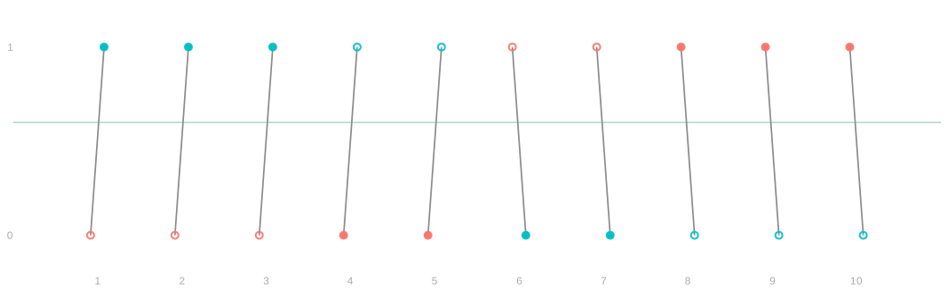
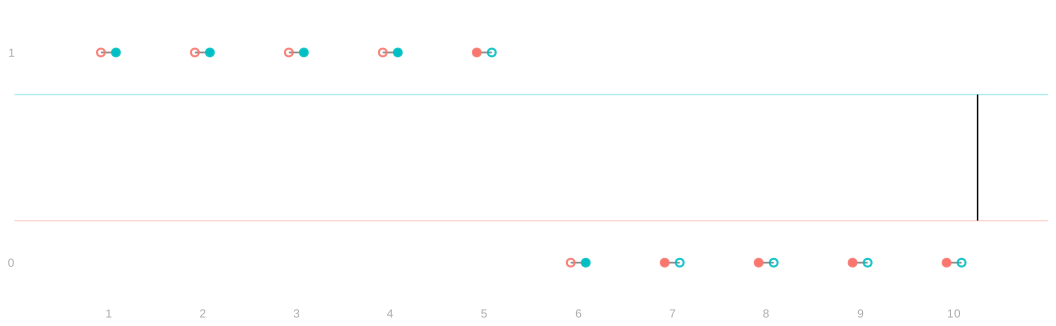
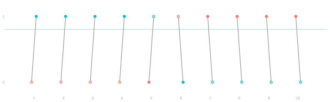
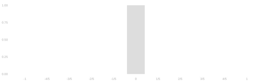
- Ten people, five assigned the prime.
- Each has one response with the prime and one without.
- Under each condition, both populations hold five salty and five fruity.
- Both have average treatment effect zero.
- The distribution of observed outcomes, as pairs, is the same.
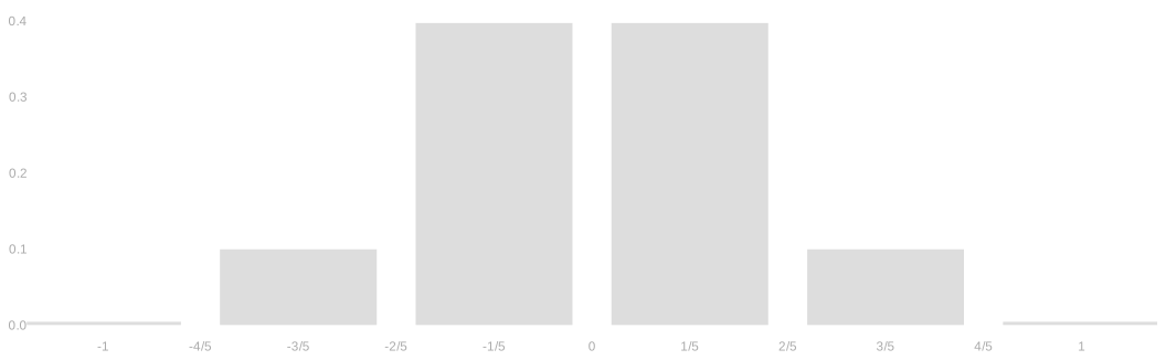
- But the spread of the estimate is different.
- In A the estimate runs from -1 to 1; in B it is zero under every assignment.
- We can estimate an upper bound on spread and overcover,
- but we can’t calibrate for exact coverage.