Power, Bias, and Coverage

Revisiting the NSW Study

Who Are These People?

$$ \newcommand{X}{} \newcommand{Y}{} % A hex digit after # inside a macro body is eaten by build-time expansion, so digit-leading hexes spell # via .

$$

Observed earnings: blue treated, red control, gray pooled.

Without replacement.

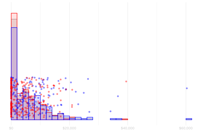
National Supported Work was a 1970s employment program for people facing serious barriers to work, including former drug users, former offenders, and young school dropouts.

Our dataset contains 445 men, of whom 185 were assigned treatment and 260 control.

• These weren’t randomly selected American men.
• They were recruited into a program intended to help people struggling to find work,
  • often beyond the difficulties associated with their demographic circumstances.

Our population for this calculation is these 445 participants.

What’s Random?

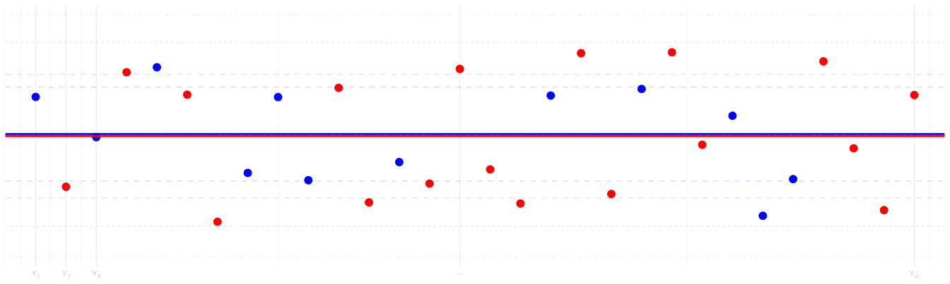
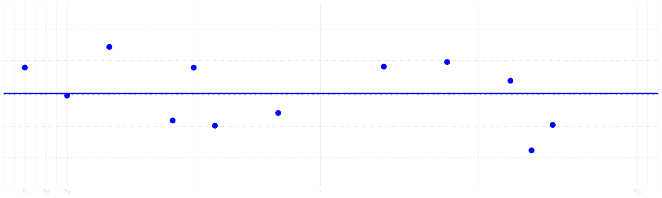
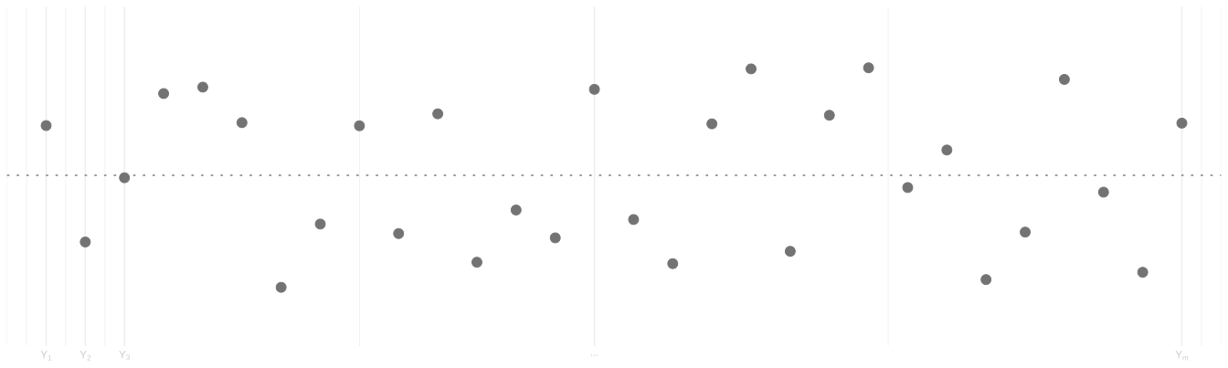
Random assignment is—the way it happened here—literally sampling the treated group¹

• Without replacement
• From the population of all study participants

Because treatment was assigned without replacement, we need to adjust the standard error we used last class.

How Many Participants?

Last class.

Without replacement: same treatment proportion.

Last class.

Without replacement: same treatment proportion.

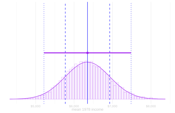
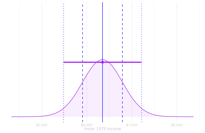
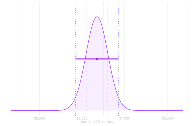
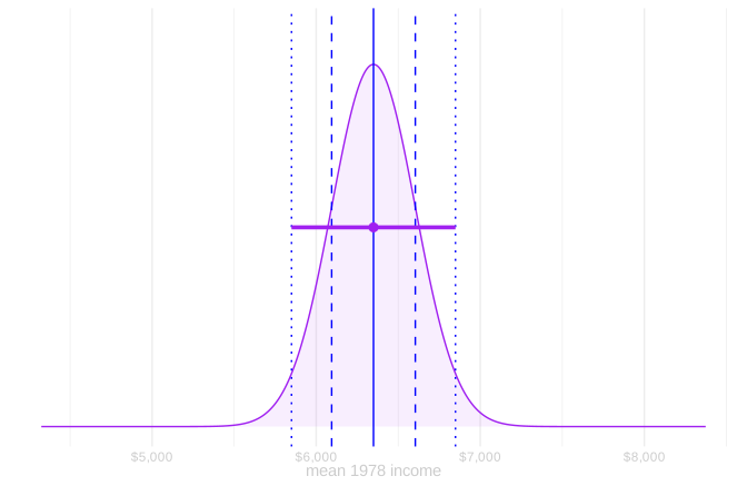
• Last class, we analyzed the study as if sampling with replacement. Our goal was a 95% interval with a half-width of 500 dollars.
• We increase the total number of participants, N, keeping the treatment fraction at about 185/445: n\approx(185/445)N.

Both times we solve for n: how many treated men it takes to get inside plus or minus 500 dollars.

\begin{aligned} \widehat{\operatorname{se}}_n&=\frac{\hat\sigma}{\sqrt n}. \\[.35em] 1.96\frac{\hat\sigma}{\sqrt n}&\le 500. \\[.35em] 1.96\hat\sigma&\le 500\sqrt n. \\[.35em] \frac{1.96\hat\sigma}{500}&\le\sqrt n. \\[.35em] \left(\frac{1.96\hat\sigma}{500}\right)^2&\le n. \end{aligned}

About 952 treated men out of 2,290 participants.

\begin{aligned} \widehat{\operatorname{se}}_n&=\frac{\hat\sigma}{\sqrt n}\sqrt{\textcolor{hotpink}{\frac{N-n}{N-1}}}. \\[.35em] 1.96\frac{\hat\sigma}{\sqrt n}\sqrt{\textcolor{hotpink}{\frac{N-n}{N-1}}}&\le500. \\[.35em] 1.96\hat\sigma\sqrt{\textcolor{hotpink}{\frac{N-n}{N-1}}}&\le500\sqrt n. \\[.35em] \frac{1.96\hat\sigma}{500}\sqrt{\textcolor{hotpink}{\frac{N-n}{N-1}}}&\le\sqrt n. \\[.35em] \left(\frac{1.96\hat\sigma}{500}\right)^2\textcolor{hotpink}{\frac{N-n}{N-1}}&\le n. \end{aligned}

About 557 treated men out of 1,340 participants.²

• At our 185 men the interval is plus or minus 1,134 dollars last class, plus or minus 868 dollars without replacement.

• Same random mechanism as the homework.

• Binary outcomes there; earnings here.

People Like Them

NSW treated men before the program (1975).

The rough CPS peers in 1975.

The same NSW treated men in 1978.

The same rough CPS peers in 1978.

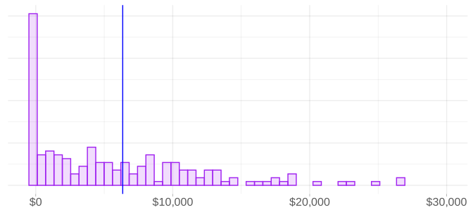
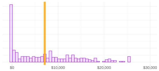
• Let’s forget that there was a control group for a minute.
• Who should we be comparing to if we want to understand whether the program worked? People like them.
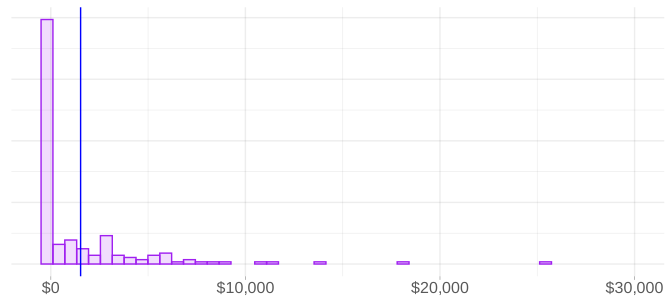
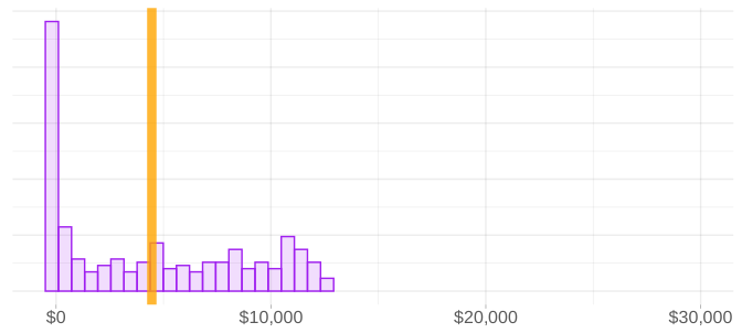
• In the Current Population Survey: Black men aged 20–35 who earned less than $12,500 in both 1974 and 1975.
  • 286 men. A rough benchmark for people sharing some of the NSW participants’ circumstances.
• Look where they started, in 1975.
• Before the program, the men assigned treatment earned about 34% of these peers’ mean earnings.
  • Mean earnings: 1,532 dollars for the NSW men and 4,455 dollars for their rough peers.
• The next picture shows the same men’s earnings in 1978.
  • Mean earnings: 6,349 dollars and 7,103 dollars.
  • The NSW men are now at about 89% of their peers’ mean.

How close would count as success?

Power Analysis

Detecting Success

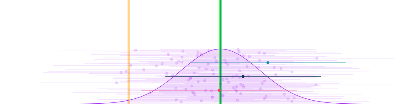
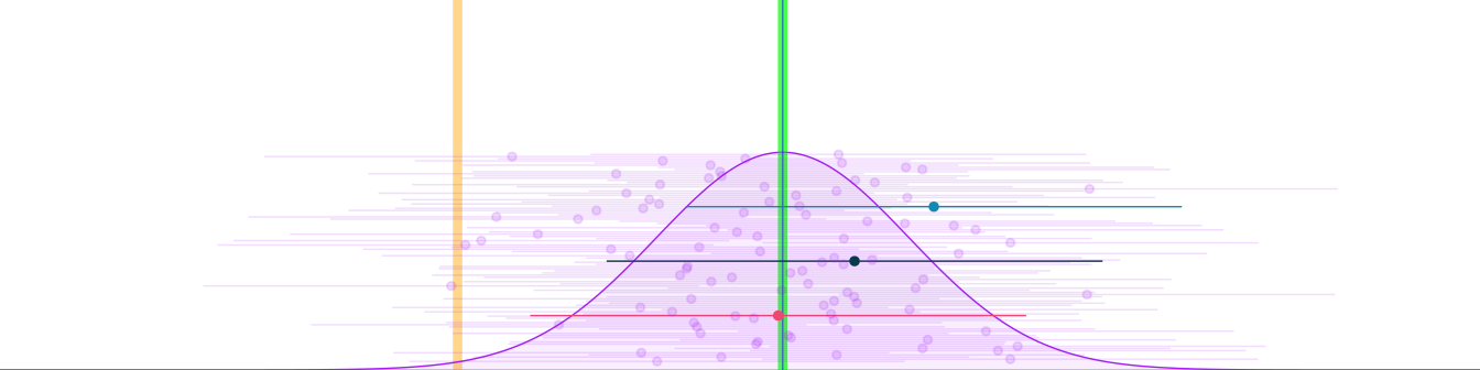
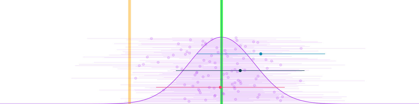
• Last class, we chose a width and called it precise enough. Now we choose it for what the study should let us say.
• Use the NSW study as a pilot to plan a larger study of the same kind.
• Suppose an agency funds a study. It calls 75% of peer earnings success: 5,327 dollars.
  • An interval estimate they’d be happy with is one that lies entirely above that standard.
• Start with a pilot, real or imagined. Then imagine running the study longer until it has the properties people ask for.
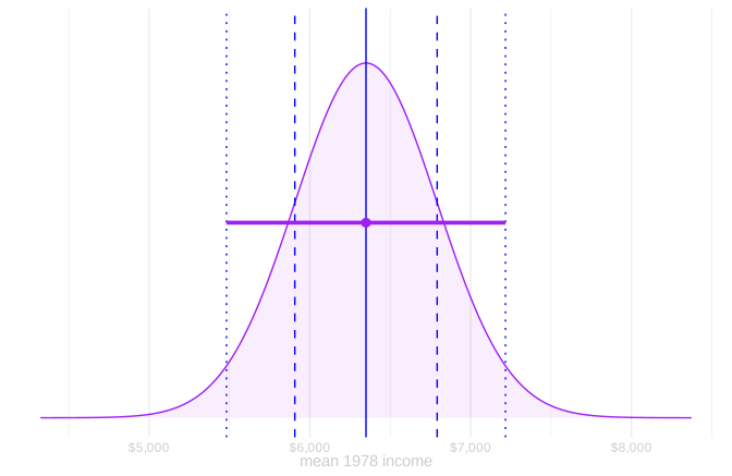
  • To size the new study, suppose the population mean is the pilot estimate, 6,349 dollars. Some people do this.³
  • Using an unbiased estimator, the center of repeated estimates coincides with the population mean.
• If that were the truth, how often would we get the evidence we need?
  • That frequency is called power. We aim for at least 80%.
  • 20% of the time, you’ll meet the standard and still not get funded. That’s randomness for you.
  • 20% is just the convention for how much uncertainty you, as a program proposer, have to stomach.

Does n=185 treated men give us enough power?
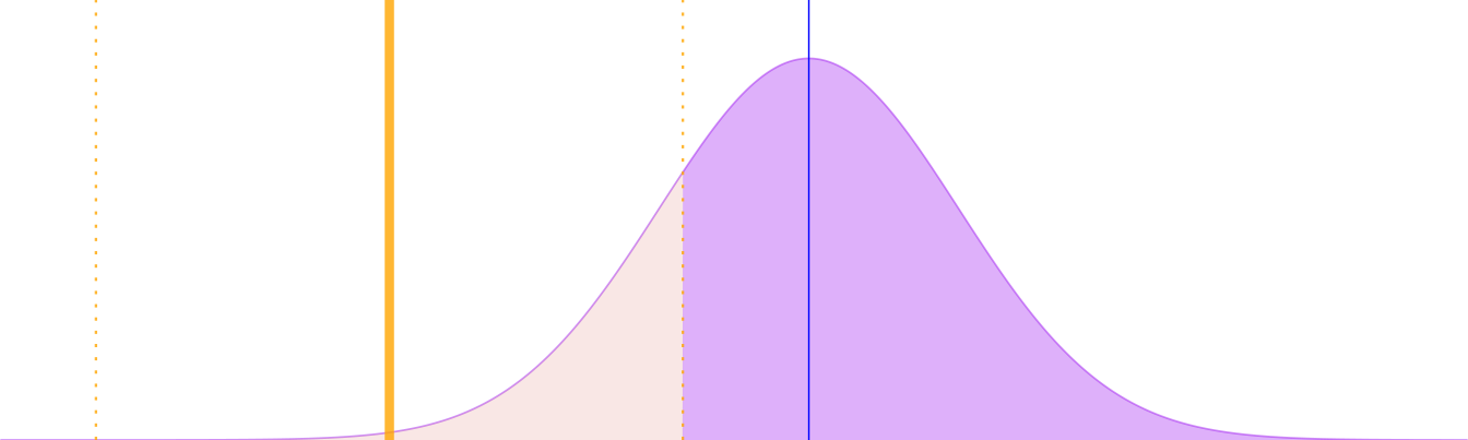
No. Only 64% of intervals lie entirely above orange.

Does n=229 treated men give us enough power?
No. Only 73% of intervals lie entirely above orange.

Does n=273 treated men give us enough power?
Yes. 80% of intervals lie entirely above orange.

Does n=546 treated men give us enough power?
Yes. And we can feel pretty confident we’ll get the evidence. 98% of intervals lie entirely above orange.

The Point of Power

• We take an interval estimate seriously as a claim about the population mean: we think it’s somewhere in here.
  • If the interval estimate is valid, we want to be happy no matter what value within it is the population mean.
  • That means its lower bound has to clear the standard.
• What does that mean?
  • Estimates in the middle of the distribution give us the evidence we want.
  • Low estimates don’t produce the evidence we want. It happens.
  • High estimates are fine.
    • You don’t need to be in the middle of the distribution.
    • You just need the interval on the right side of the standard.

Power Calculation

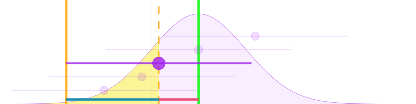
• How much data do we need to get that evidence 80% of the time?
  • The assumed mean and the agency’s standard stay fixed.
  • More data reduces the standard error.
• The interval requirement
  • Its lower bound is 1.96 standard errors below the estimate.
  • The estimate therefore has to be 1.96 standard errors above the standard.
• The power requirement
  • That means we need 80% of estimates to be at least 1.96 standard errors above the standard.
  • That means the sampling distribution’s 20th percentile—0.84 standard errors below the mean—has to be at least 1.96 standard errors above the standard.
• The sample-size requirement

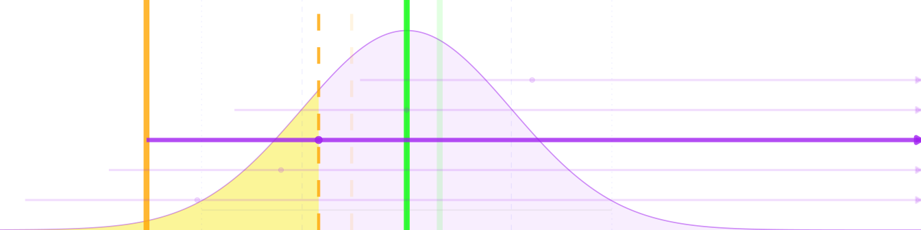
• We only need a lower bound to show that mean earnings exceed the standard.
  • An upper bound cannot help us show that.
  • So we let the interval extend upward without limit.
• A one-sided 95% interval can miss the mean only by starting too high.
  • The full 5% failure probability goes to that case, instead of 2.5% on each side.
  • Its lower bound is 1.65 standard errors below the estimate.
  • The estimate therefore has to be 1.65 standard errors above the standard.
• We still want that evidence 80% of the time.
  • The sampling distribution’s 20th percentile—0.84 standard errors below the mean—has to be at least 1.65 standard errors above the standard.
• We solve the same equation with the new lower bound.

\begin{aligned} \text{Mean} - \textcolor{#ef476f}{0.84\,\text{SE}} &= \text{Standard} + \textcolor{#118ab2}{1.96\,\text{SE}}, \\[.35em] \text{and therefore}\qquad \text{Mean} &= \text{Standard} + 2.80\,\text{SE}. \end{aligned}

Substituting our standard error formula and rearranging:

\begin{aligned} 2.80\frac{\hat\sigma}{\sqrt n}\sqrt{\textcolor{hotpink}{\frac{N-n}{N-1}}}&\le\text{Mean}-\text{Standard}. \\[.35em] \left(\frac{2.80\hat\sigma}{\text{Mean}-\text{Standard}}\right)^2\textcolor{hotpink}{\frac{N-n}{N-1}}&\le n. \end{aligned}

To meet this standard, we choose our sample size so that the gap between the assumed mean and the standard is at least 2.80 standard errors.

For n satisfying that:⁴ n=273 treated men, with 80% of intervals entirely above orange.

\begin{aligned} \text{Mean} - \textcolor{#ef476f}{0.84\,\text{SE}} &= \text{Standard} + \textcolor{#118ab2}{1.65\,\text{SE}}, \\ \text{and therefore}\qquad \text{Mean} &= \text{Standard} + 2.49\,\text{SE}. \end{aligned}

To get that evidence 80% of the time, we choose our sample size so that the mean is at least 2.49 standard errors above the standard—about 2.5.

The 95% coverage and 80% power levels are conventions, including in clinical-trial guidance (FDA/ICH E9, §3.5).

Detecting Futility

• Sometimes we want power to find evidence of futility.

  • Suppose the agency requires full catch-up with the comparison group.
  • We again suppose the population mean is the pilot estimate, 6,349 dollars.
  • This is the mirror image of detecting success.

• The interval requirement

  • The evidence we want for stopping is an interval entirely below the standard.
  • Its upper bound is 1.96 standard errors above the estimate.
  • The estimate therefore has to be 1.96 standard errors below the standard.

• The power requirement

  • We want 80% of estimates to be at least 1.96 standard errors below the standard.
  • The sampling distribution’s 80th percentile—0.84 standard errors above the mean—has to be at least 1.96 standard errors below the standard.

• The sample-size requirement

  \begin{aligned} \text{Mean} + \textcolor{#ef476f}{0.84\,\text{SE}} &= \text{Standard} - \textcolor{#118ab2}{1.96\,\text{SE}}, \\ \text{and therefore}\qquad \text{Mean} &= \text{Standard} - 2.80\,\text{SE}. \end{aligned}

We choose our sample size so that the gap between the standard and the assumed mean is at least 2.80 standard errors.

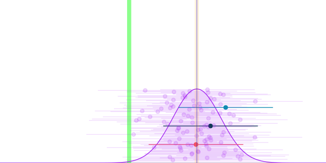
n=501 treated men: 80% of intervals lie entirely below orange.

The Power of Bias

• Bias gives you power against the truth. It’s not a metaphor.

  • Coverage is how often an interval contains the truth.
  • Power against the truth is how often it misses.

  \underset{\text{coverage}}{\Pr(\text{covers green})} \;=\; 1-\underset{\text{power}}{\Pr(\text{doesn't cover green})}

• Power isn’t really about the relationship between the green line and the orange one.

  • It’s about the relationship between the blue line—the sampling distribution’s center—and any other line.
  • Power is just how often intervals from that sampling distribution don’t cross a line.
  • The procedure doesn’t know which line is the estimand and which is the standard.

• As the sampling distribution shifts away from the estimand…

  • …our intervals shift with it.
  • Fewer intervals cover the estimand, so coverage falls.

When the bias has increased enough for the center of our estimates to reach the CPS mean, this happens.

• What was 80% power has become 20% coverage.
  • Before the shift, 80% of intervals lay entirely below the CPS mean.
  • After the shift, 80% of intervals lie entirely above the NSW mean.
  • So we have only 20% coverage—or equivalently 80% power against the NSW mean.
• How do we get this kind of bias? It’s easy. We survey the wrong population.
  • We want to estimate the NSW mean.
  • If we survey CPS people instead, our estimates are centered on the CPS mean.

Bad Comparisons

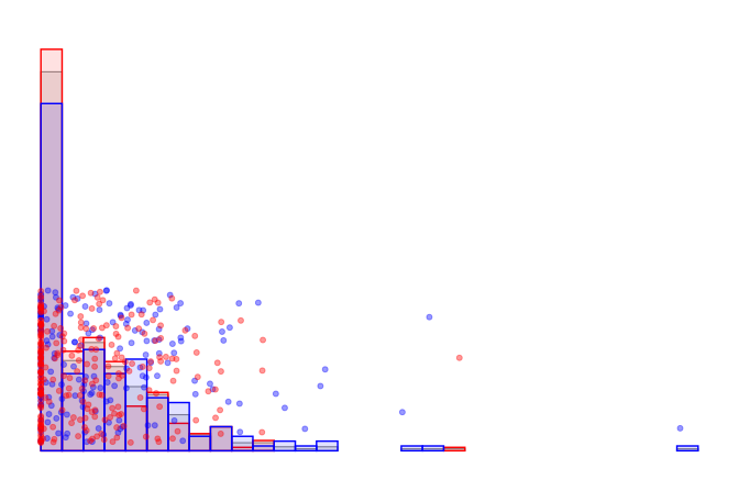
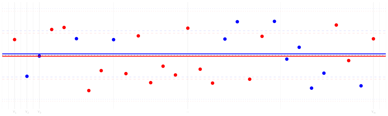
Observed NSW earnings: blue treated, red controls.

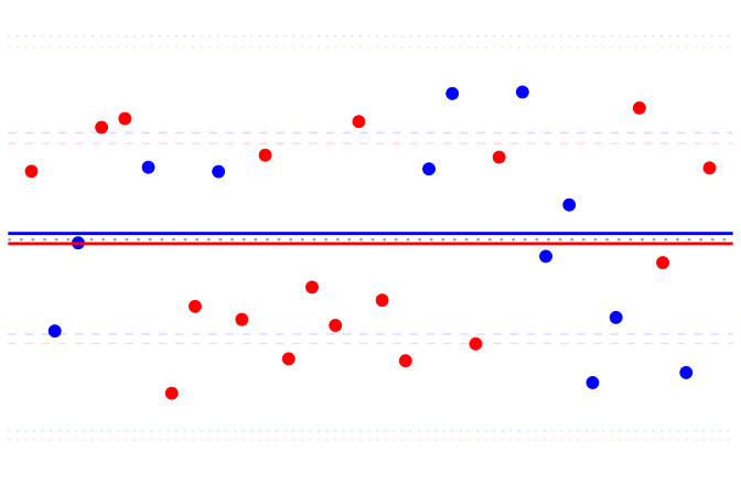
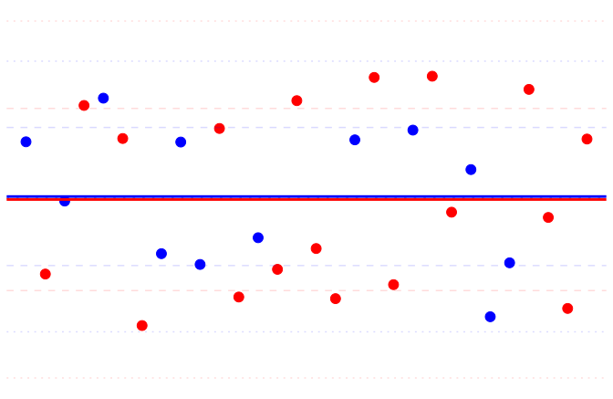
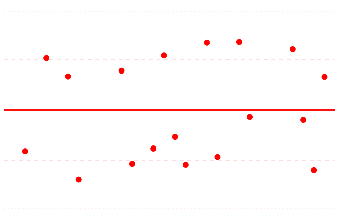
Assignment schematic: now keep the controls.

• How could we get that biased picture in this study? Think about the controls.
• The NSW controls estimate the NSW population’s mean earnings without the program.
  • Random assignment gives us a sample of its untreated outcomes: 260 of the 445 participants.
• More observations could improve precision, so consider sampling people outside the study.
  • Our CPS records are a sample from a subpopulation of Black men aged 20–35 with low recent earnings.
  • If we take a simple random sample from the CPS subpopulation, the sample mean is unbiased …
    • … for that subpopulation’s mean. Not the NSW population’s.
    • Using it for the NSW population’s untreated mean introduces bias if the two population means differ.

Imperfect Comparisons

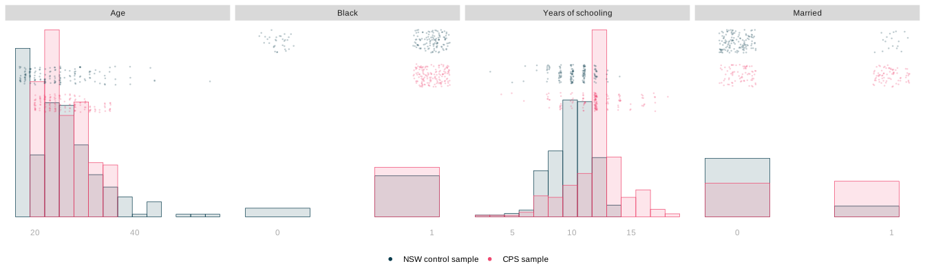
• Selecting for some features still leaves differences in composition.
  • We selected for age, race, and recent earnings, but even the age and race distributions are poorly matched.
  • Other features, including schooling and marriage, also differ.
• Differences in composition can change mean earnings.
  • For example, marriage wasn’t a selection criterion: 15.4% of the NSW control sample is married, compared with 51.4% of the CPS sample.
  • Hold average earnings among married and unmarried CPS men fixed; replace the CPS married share with the NSW control share.
    • The reweighted mean is 7,462 dollars, 359 dollars above the CPS sample mean of 7,103 dollars.
• The real question is not whether the populations differ, but whether there’s enough bias that your coverage is ruined.
  • Use the observed NSW controls and CPS records as two populations with known means.

The Bigger, the Worse

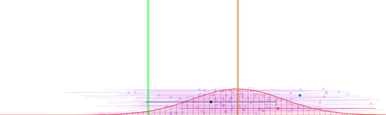
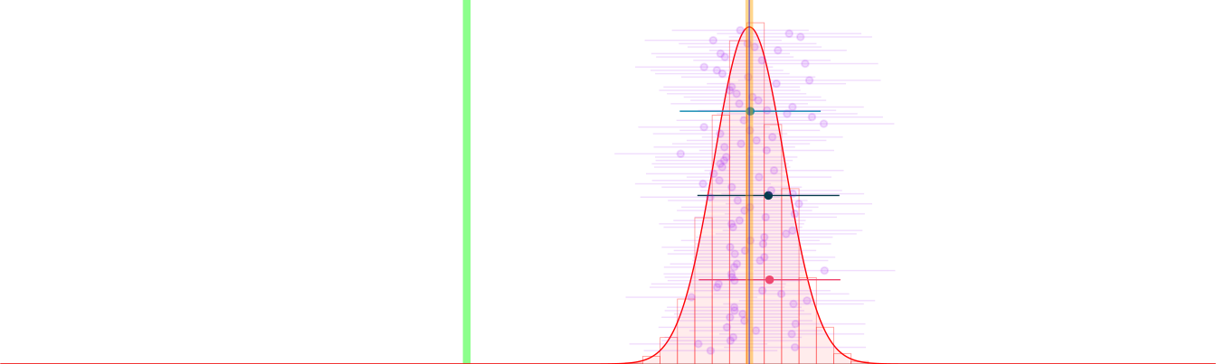
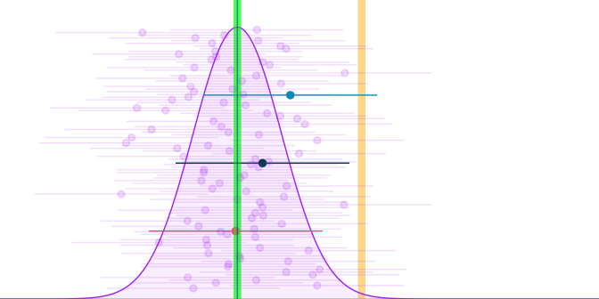
n = 30. Intervals containing green in 2,000 simulated studies: 51%.

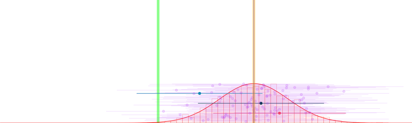
n = 60. Intervals containing green in 2,000 simulated studies: 19%.

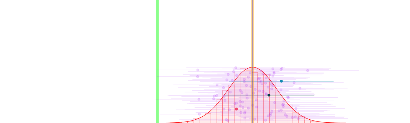
n = 120. Intervals containing green in 2,000 simulated studies: 2%.

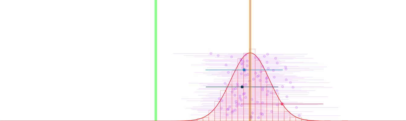
n = 185. Intervals containing green in 2,000 simulated studies: 0 of 2,000.

n = 500. Intervals containing green in 2,000 simulated studies: 0 of 2,000.

• We’re sampling from the CPS population to estimate the NSW control population’s mean.

  • The sampling distribution is centered on the CPS mean.

• A bigger sample gives us a narrower interval around the wrong mean.

  • The bias in dollars stays fixed, but it grows relative to the standard error.
  • As the intervals shrink, fewer contain the NSW control population’s mean.

• We just gave ourselves power against the truth.

  \text{coverage}=1-\Pr(\text{interval excludes the truth}).

• How much bias does it take to do this?

Calculating Coverage

Set Up

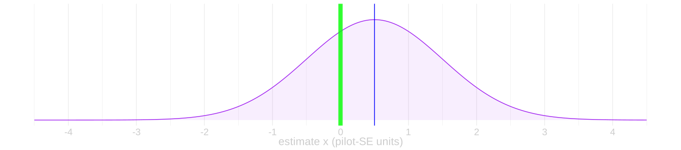
• Suppose a closer comparison leaves bias of half a pilot standard error. This is an illustrative assumption.
  • In pilot-SE units, the truth is \mu=0 and the center of the estimates is \tilde\mu=0.5.
• We’re going to calculate that estimator’s coverage rate. Approximately. We’ll make some simplifications.
• We’ll act as if the normal approximation to the sampling distribution were perfect.
• We’ll use the estimator’s actual standard error, \sigma, to form each interval: \hat\mu \pm 1.96\sigma.

Which Estimates Hit The Target?

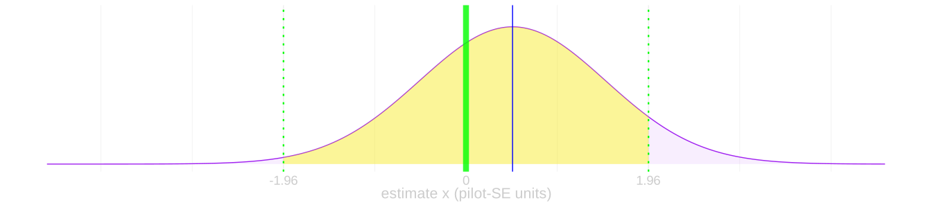
• Let’s think about things from the target’s perspective. The solid green line.
  • Give it arms the same length as our intervals have: out to the dotted green lines.
• An interval’s arms reach the target if and only if the target’s arms reach that interval’s center.
• We integrate the sampling distribution’s density between the target’s arms.

\text{coverage} = \int_{\mu-1.96\sigma}^{\mu+1.96\sigma} f(x) dx \qqtext{ where } f(x)=\frac{1}{\sqrt{2\pi} \sigma} e^{-\frac{(x-\tilde\mu)^2}{2\sigma^2}}

Which point estimates produce intervals that hit the target? Ask for the region and point to the shaded area. This is a spoken question while working through the picture, not a request for students to write an answer at their desks. The normal density formula is supplied; they do not need to recall it.

A Standard Normal Area

• Now we’ll rewrite our coverage as an integral of the standard normal density. R can calculate that density’s areas.
• To do it, we’re going back to intro calculus. We’re making a substitution u=(x-\tilde\mu)/\sigma.

• This means we have to change the limits.
  • As x goes from \mu-1.96\sigma to \mu+1.96\sigma, u goes from -1.96-(\tilde\mu-\mu)/\sigma to 1.96-(\tilde\mu-\mu)/\sigma.
• And make a substitution into the integrand.
  • For (x-\tilde\mu)^2/\sigma^2, we substitute u^2.
• And multiply by dx/du so we get to integrate over u.
  • x= u\sigma + \tilde\mu so dx=\sigma du. The two \sigma factors cancel.

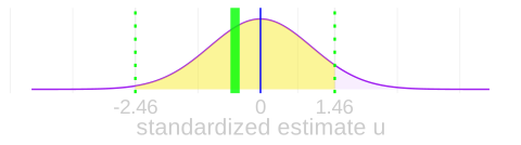
\begin{aligned} \text{coverage} &= \int_{\mu-1.96\sigma}^{\mu+1.96\sigma} \frac{1}{\sqrt{2\pi} \sigma} e^{-\frac{(x-\tilde\mu)^2}{2\sigma^2}} dx \\ &= \int_{-1.96-(\tilde\mu-\mu)/\sigma}^{1.96-(\tilde\mu-\mu)/\sigma} \frac{1}{\sqrt{2\pi} \sigma} e^{-\frac{u^2}{2}} \sigma du \\ &= \int_{-1.96-(\tilde\mu-\mu)/\sigma}^{1.96-(\tilde\mu-\mu)/\sigma} \textcolor{blue}{\frac{1}{\sqrt{2\pi}} e^{-\frac{u^2}{2}}} du \end{aligned}

Subtracting the center and dividing by the standard error gives a standard normal variable. The two pictures show the same probability in different coordinates. Carry the substitution yourself. Point out the new endpoints, the exponent becoming u squared, and the two sigma factors canceling. This is not independent calculus work. The normal density formula was supplied; I’m not expecting you to have that memorized, but it does come in handy from time to time.

Summary and Generalization

Bias of half a standard error: \operatorname{pnorm}(1.46)-\operatorname{pnorm}(-2.46) = 92.09\% coverage.

Same comparison and bias, sixteen times as much data: if SE scales as 1/\sqrt n, it falls to one-quarter. Bias is now two SEs: \operatorname{pnorm}(-0.04)-\operatorname{pnorm}(-3.96) = 48.40\% coverage.

• Coverage depends on the bias relative to the standard error.
• It’s an integral of the standard normal density over the range \pm 1.96 -\text{bias}/\text{se}.
• The R function call pnorm(x) calculates that integral from -\infty to x. All we need to do is subtract.

Math Version

\small{ \begin{aligned} \text{coverage} &=\int_{-1.96-\frac{\text{bias}}{\text{se}}}^{+1.96-\frac{\text{bias}}{\text{se}}} \frac{1}{\sqrt{2\pi}} e^{-\frac{u^2}{2}} du \\ &= \int_{-\infty}^{+1.96-\frac{\text{bias}}{\text{se}}} \frac{1}{\sqrt{2\pi}} e^{-\frac{u^2}{2}} du \ - \ \int_{-\infty}^{-1.96-\frac{\text{bias}}{\text{se}}} \frac{1}{\sqrt{2\pi}} e^{-\frac{u^2}{2}} du \end{aligned} }

R Version

coverage = function(bias.over.se) {  pnorm(1.96 - bias.over.se) - pnorm(-1.96 - bias.over.se)  }

Examples

 
 
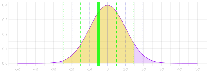
\frac{\text{bias}}{\text{se}} = \frac{1}{2} \quad \implies \quad \text{coverage} = 92\%

 
 
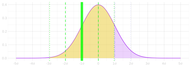
\frac{\text{bias}}{\text{se}} = 1 \quad \implies \quad \text{coverage} = 83\%

 
 
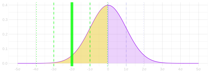
\frac{\text{bias}}{\text{se}} = 2 \quad \implies \quad \text{coverage} = 48\%

 
 
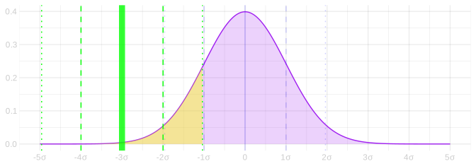
\frac{\text{bias}}{\text{se}} = 3 \quad \implies \quad \text{coverage} = 15\%

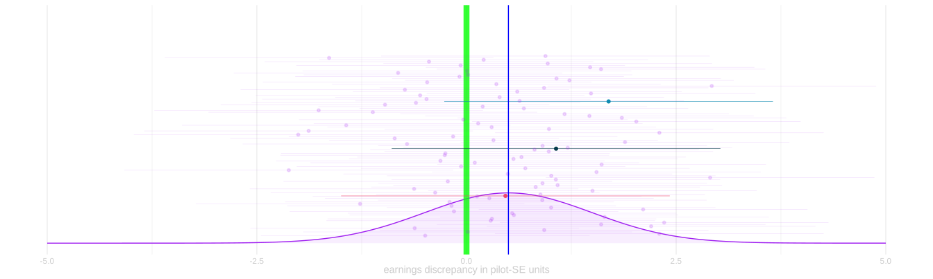
• Suppose we’ve got bias, but only a little bit.

• We’re doing a pilot study with sample size n=100.

• And we’re sure that our estimator’s absolute bias is less than half its standard error.

• Question 1. What’s the coverage of our 95% confidence intervals?

• A. At least 92%.

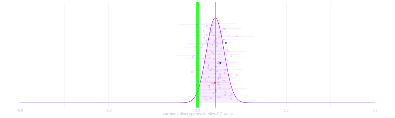
• Now suppose we’re doing a follow-up study with sample size n=1600.
• And we’re using the same estimator. Bias is the same.
• Question 2. What’s the coverage of our 95% confidence intervals?
• Assume our estimator’s standard error is proportional to \sqrt{1/n}.
  • This is the relation we used for independent sample means last class.
  • That means it’ll be \sqrt{1/1600} \ / \ \sqrt{1/100}=\sqrt{1/16}=1/4 of what it was in the pilot study.

• A. At least 48%. Here’s why. \text{If } \ \frac{\abs{\text{bias}}}{\text{pilot se}} \le 1/2 \ \text{ and } \ \text{follow-up se} = \frac{\text{pilot se}}{4}, \ \text { then } \ \frac{\abs{\text{bias}}}{\text{follow-up se}} = 4 \times \frac{\abs{\text{bias}}}{\text{pilot se}} \le 2.

The Coverage Curve

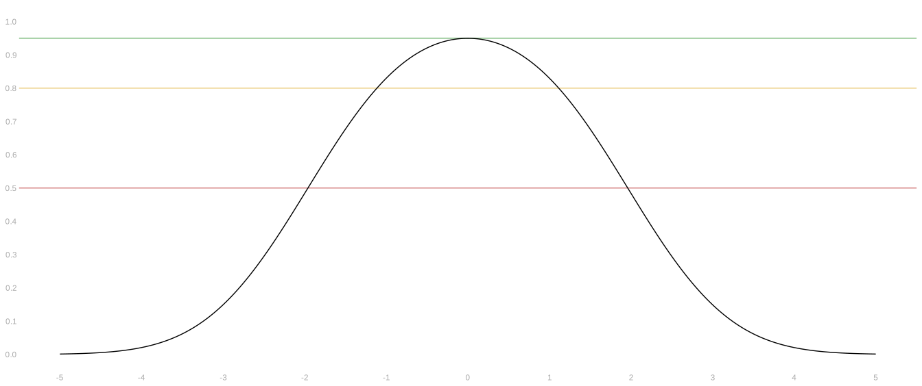
Reference points: nominal · questionable · coinflip

Calculating Power

• Remember: two-sided power to rule out a line is one minus the fraction of intervals that cover that line.
• We already know how to calculate it. Replace bias in SE units by the distance from that line to the estimator’s center.

\text{two-sided power}=1-\text{coverage}(d),\qquad d=\frac{\text{estimator center}-\text{reference line}}{\text{se}}.

• For success or futility, count only the tail on the side that answers the decision.
• It is still the same normal-area calculation.

Finding People Like Them

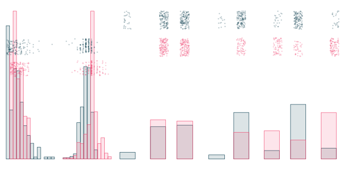
Age · Years of schooling · Black · Hispanic · Married · Finished high school.

NSW controls · rough CPS peers

About 80% power against orange at 501 men.

• We learned how to make a study more powerful by increasing its precision.
• That worked. It also made our persistent bias increasingly consequential.
• We made a pretty reasonable attempt to find “people like them.”
• One characteristic we hadn’t thought much about changed the benchmark.

This is why we do experiments. Stay tuned.

We’ll return to these two NSW outcome lists when we formalize potential outcomes and ask what the randomized comparison tells us about the program.

What If They Were Never Exactly Equal?

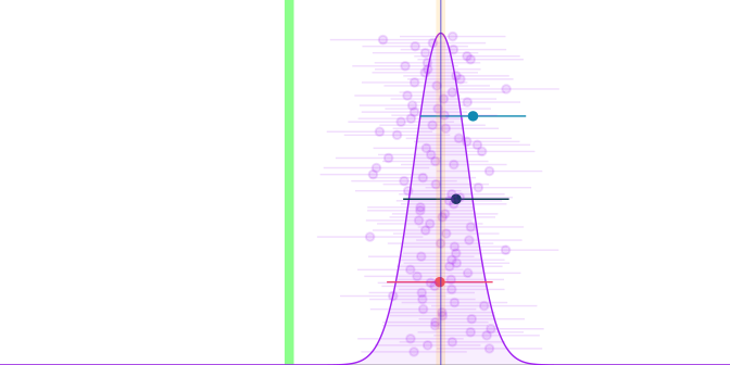
• Outside physics and randomized experiments, two things are never exactly equal.
• Testing whether they are only tells you whether you have enough power to say they aren’t.

McShane, Gal, Gelman, Robert, and Tackett, Abandon Statistical Significance, §2.2

Appendix

The simulated populations

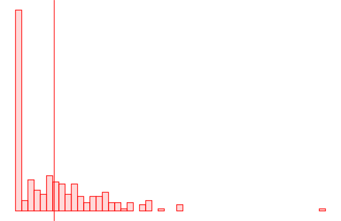
Observed NSW controls (260).

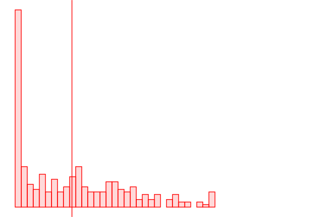
Observed CPS subgroup (286).

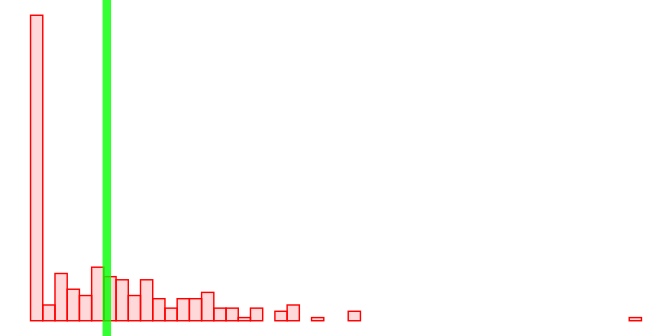
The target: our constructed population of NSW controls. Its known mean is 4,555 dollars.

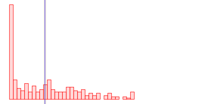
The data: samples with replacement from the CPS subgroup’s empirical distribution. Its mean is 7,103 dollars.

• That was an illustration of what might happen, not what actually happened.
  • Because we don’t know.
  • That’s real data for you.
• What we really want to be analyzing is fake data.
  • To keep it interesting, let’s make it look pretty real.
• The target: our constructed population of NSW controls. Its known mean is 4,555 dollars.
• Is this legit?
  • It’s a population with a mean and characteristics for our CPS subpopulation to imitate.
    • Imperfectly.
  • Hitting this constructed target does not guarantee hitting the real NSW population’s untreated mean.
    • If it did, we wouldn’t have a precision problem to start with.
• The CPS mean was our benchmark.
  • It is now the center of the estimates we’ll get from those samples: 7,103 dollars, compared with the target at 4,555 dollars.
• Both populations are built from observed data.
  • We know both means inside this simulated world.
• For each study, draw n CPS records with replacement and form the sample mean plus or minus 1.96 estimated standard errors.
  • How often does that interval contain the NSW control population’s mean?

The n on both sides

• Recognize the problem.
  • The pink factor leaves an n on both sides of the condition.
• Recognize the approximation.
  • That factor is less than one, so dropping it only asks for more men.
  • An overestimate is the safe direction for a sample size.
• Then recognize that you can do better.
  • We hold the treatment fraction at f=185/445, so N=n/f.

\begin{aligned} \textcolor{hotpink}{\frac{N-n}{N-1}}&=\frac{n/f-n}{n/f-1}. \\[.35em] &=\frac{n-nf}{n-f}. \\[.35em] &=\frac{n(1-f)}{n-f}. \end{aligned}

• Put that back in and divide both sides by n.

\begin{aligned} \left(\frac{1.96\hat\sigma}{500}\right)^2\frac{n(1-f)}{n-f}&\le n. \\[.35em] \left(\frac{1.96\hat\sigma}{500}\right)^2\frac{1-f}{n-f}&\le 1. \\[.35em] \left(\frac{1.96\hat\sigma}{500}\right)^2(1-f)&\le n-f. \\[.35em] \left(\frac{1.96\hat\sigma}{500}\right)^2(1-f)+f&\le n. \end{aligned}

• It was a linear equation the whole time.
  • Up to rounding to a whole number of men.
  • For power, swap the 1.96 for 2.80 and the 500 dollars for the gap.

Footnotes

1. Think of two outcome lists for the same NSW participants: earnings with the program and earnings without it. Random assignment reveals a sample from each list. We’ll formalize this later using potential outcomes.

2. The pink factor leaves an n on both sides. Drop it and you get an overestimate. Or we can solve for n in terms of the treatment fraction and everything else, easily: appendix.

3. Andrew Gelman and John Carlin (2014), Beyond Power Calculations: Assessing Type S (Sign) and Type M (Magnitude) Errors, p. 642. They describe using a previous study’s estimated effect in prospective power planning and caution that preliminary estimates may exaggerate effects.

4. Same n on both sides as before, and it solves the same way: appendix.