Normal Approximation: the Proof

Tools

Integration by parts

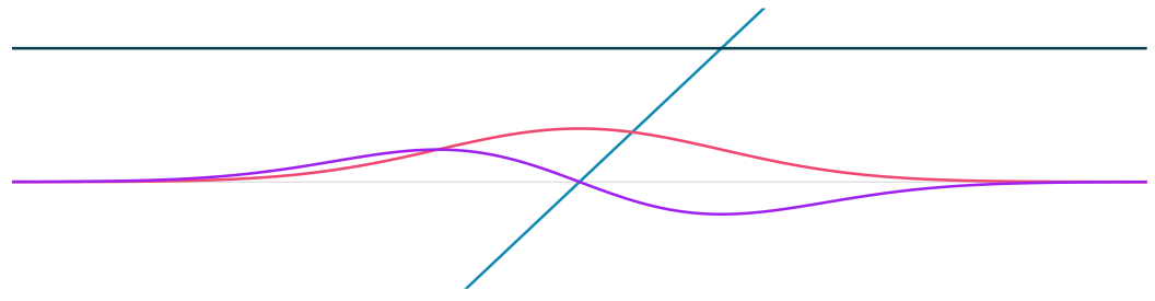
I can never remember this formula, so I start with the product rule for derivatives. (\textcolor{#118AB2}{u}\textcolor{#EF476F}{v})'=\textcolor{#073B4C}{u'}\textcolor{#EF476F}{v}+\textcolor{#118AB2}{u}\textcolor{#A020F0}{v'} \qqtext{so rearranging} \textcolor{#073B4C}{u'}\textcolor{#EF476F}{v} = (\textcolor{#118AB2}{u}\textcolor{#EF476F}{v})'-\textcolor{#118AB2}{u}\textcolor{#A020F0}{v'}. Integrating, we get the integration by parts formula. \int_a^b \textcolor{#073B4C}{u'(x)}\textcolor{#EF476F}{v(x)}\,dx =\textcolor{#118AB2}{u(x)}\textcolor{#EF476F}{v(x)} \mid_a^b-\int_a^b \textcolor{#118AB2}{u(x)}\textcolor{#A020F0}{v'(x)}\,dx. Often the boundary term is zero: \textcolor{#118AB2}{u(x)}\textcolor{#EF476F}{v(x)} is the same at both ends. This gives us a simple rule: flip the derivative, flip the sign. \int_{a}^{b}\textcolor{#073B4C}{u'(x)}\textcolor{#EF476F}{v(x)}\,dx =-\int_{a}^{b}\textcolor{#118AB2}{u(x)}\textcolor{#A020F0}{v'(x)}\,dx. Why zero? Today, it’s because we’ll be integrating from -\infty to \infty. And \textcolor{#118AB2}{u(x)}\textcolor{#EF476F}{v(x)} \to 0 as x \to \pm\infty.

Standardization

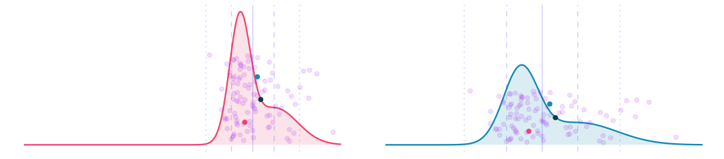
Today, we’re going to be working with standardized averages.
What does standardized mean?
- Centered. We subtract its expected value.
- Scaled: We divide by its standard deviation.
We can write a standardized average of independent random variables with the same distribution as a sum of random variables with standard deviation 1/\sqrt{n}.

\textcolor{#118AB2}{W} =\frac{\textcolor{#EF476F}{\hat\mu}-\mu}{\sigma/\sqrt n} =\frac{\textcolor{#A020F0}{\frac 1n\sum_{i=1}^{n}(Y_i-\mu)}}{\textcolor{#A020F0}{\sigma/\sqrt n}} =\sum_{i=1}^{n}\textcolor{#A020F0}{X_i}\quad \text{with}\quad \operatorname{sd}(\textcolor{#A020F0}{X_i}) =\frac{\operatorname{sd}(\textcolor{#A020F0}{Y_i-\mu})}{\textcolor{#A020F0}{\sigma\sqrt n}} =\frac{\sigma}{\sigma\sqrt n} =\frac{1}{\sqrt n}.

Swapping in independent copies

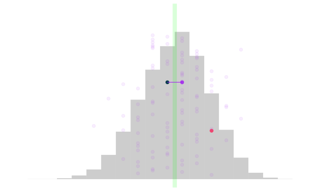
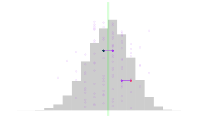
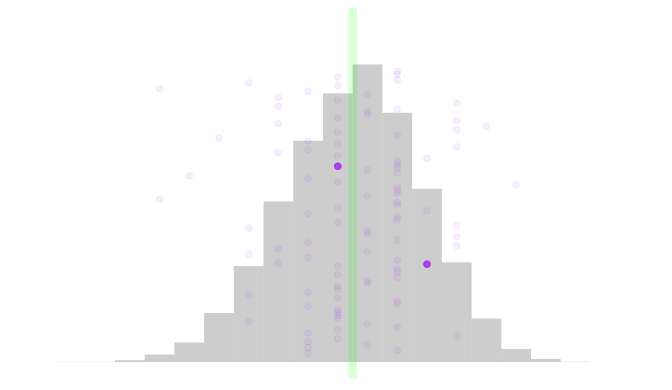
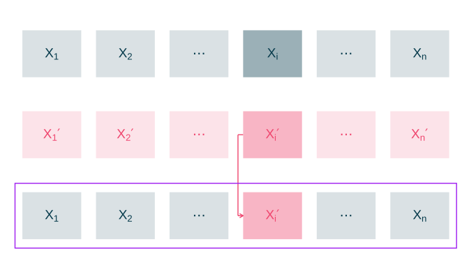
One person runs a survey. Another person independently runs the same survey, the same way.
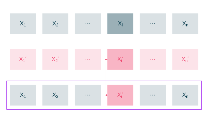
- We say their response sequence \textcolor{#EF476F}{X_1' \ldots X_n'} is an independent copy of yours.
- Same survey design, same population, same response distribution.
We do the swap. What changes?

\begin{aligned} \textcolor{#073B4C}{W}&=\textcolor{#073B4C}{X_1}+\cdots+\textcolor{#073B4C}{X_i}+\cdots+\textcolor{#073B4C}{X_n}&&\text{your original average}\\ \textcolor{#A020F0}{W_i'}&=\textcolor{#073B4C}{X_1}+\cdots+\textcolor{#EF476F}{X_i'}+\cdots+\textcolor{#073B4C}{X_n}&&\text{your post-swap average}\\ \textcolor{#073B4C}{W}-\textcolor{#A020F0}{W_i'}&=\textcolor{#073B4C}{X_i}-\textcolor{#EF476F}{X_i'}&&\text{the difference}. \end{aligned}

Does the value change? A little. The difference has standard deviation \textcolor{#118AB2}{\sqrt{2/n}}.
Does the distribution change? Not at all.

Bounding a product by cubes

For nonnegative a and b, the product ab^2 is at most a weighted average of their cubes.

ab^2\le\frac{a^3+2b^3}{3}.

\frac{a^3+2b^3}{3}-ab^2 \overset{\mathtip{\small{\text{?}}}{\text{Expand the product and collect terms.}}}{=}\frac{(a-b)^2(a+2b)}{3} \overset{\mathtip{\small{\text{?}}}{\text{Both factors are nonnegative when }a,b\ge 0.}}{\ge}0.
For centered \textcolor{#073B4C}{A} and an independent copy \textcolor{#EF476F}{B}, this bounds the average change from a swap.

\mathbb E\{|\textcolor{#073B4C}{A}|(\textcolor{#073B4C}{A}-\textcolor{#EF476F}{B})^2\} \le2\mathbb E|\textcolor{#073B4C}{A}|^3.

\begin{aligned} \mathbb E\{|\textcolor{#073B4C}{A}|(\textcolor{#073B4C}{A}-\textcolor{#EF476F}{B})^2\} &\overset{\mathtip{\small{\text{?}}}{\text{Expand the square and use independence in the cross term.}}}{=}\mathbb E|\textcolor{#073B4C}{A}|^3 -2\mathbb E(|\textcolor{#073B4C}{A}|\textcolor{#073B4C}{A})\underbrace{\mathbb E\textcolor{#EF476F}{B}}_{0} +\mathbb E(|\textcolor{#073B4C}{A}|\textcolor{#EF476F}{B}^2)\\ &\overset{\mathtip{\small{\text{?}}}{\begin{gathered}\mathbb E\textcolor{#EF476F}{B}=0.\\\text{Apply the product bound to }|\textcolor{#073B4C}{A}|\,|\textcolor{#EF476F}{B}|^2.\end{gathered}}}{\le}\mathbb E|\textcolor{#073B4C}{A}|^3+ \frac{\mathbb E|\textcolor{#073B4C}{A}|^3+2\mathbb E|\textcolor{#EF476F}{B}|^3}{3}\\ &\overset{\mathtip{\small{\text{?}}}{\text{The copy has the same absolute third moment.}}}{=}2\mathbb E|\textcolor{#073B4C}{A}|^3. \end{aligned}

Taylor approximation

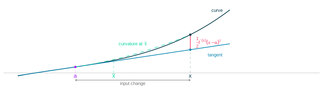
A first-order Taylor approximation replaces a curve by its tangent line.

f(\textcolor{#073B4C}{x})\approx f(\textcolor{#A020F0}{a})+(\textcolor{#073B4C}{x}-\textcolor{#A020F0}{a})f'(\textcolor{#A020F0}{a}).
Curvature controls the gap between the curve and its tangent. The matching quadratic uses the curvature at an intermediate point.

\begin{aligned} f(\textcolor{#073B4C}{x})-f(\textcolor{#A020F0}{a})-(\textcolor{#073B4C}{x}-\textcolor{#A020F0}{a})f'(\textcolor{#A020F0}{a}) &=\frac12 f''(\tilde x)(\textcolor{#073B4C}{x}-\textcolor{#A020F0}{a})^2\\ &\quad\text{where }\textcolor{#06D6A0}{\tilde x}\text{ lies between }\textcolor{#A020F0}{a}\text{ and }\textcolor{#073B4C}{x}. \end{aligned}

The normal is universal

The normal is stable

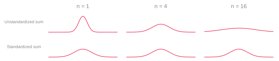
The average of normals is normal.
If averaging settles toward a shape, averaging again must leave that shape unchanged.
- The normal has that property. After standardizing, the bottom row stays the same.
- Could this be why averages approach the normal?

Averaging makes things normal

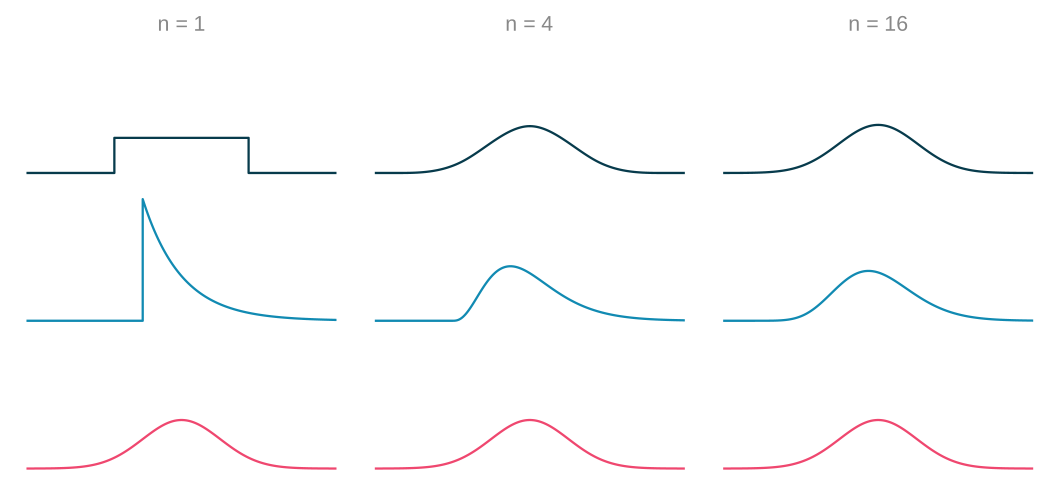
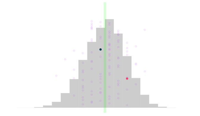
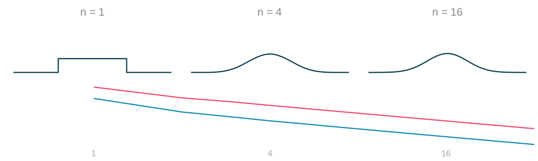
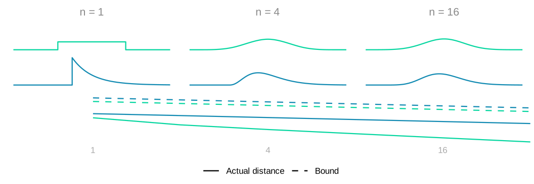
We look at standardized averages for three distributions. W_n=\frac{\sum_{i=1}^n(Y_i-\mu)}{\sigma\sqrt n}=\sum_{i=1}^nX_i.

As we increase our sample size, the averages start to look more normal.

How we’ll show this

Characterization. The normal’s signature is zero.
Approximation. Sums have signatures close to zero.
Continuity. Close signatures mean close distributions.

The same strategy works elsewhere

Find a property that identifies the object we want.
Show that our objects approximately have that property.
Show that approximately having the property makes them close to the object we want.

Wishful thinking: a strategy

Wishful thinking gives us a next step before we can see the whole proof.

What do we want? What do we have? Can we make them the same thing?
- For standardization, we had Y with mean \mu and standard deviation \sigma. We wanted mean zero and standard deviation one.

\underbrace{W=a+bY\ (b>0)}_{\text{what we try}} \qquad \underbrace{a+b\mu=0\quad\text{and}\quad b\sigma=1}_{\text{what it must do}} \qquad\Longrightarrow\qquad W=\frac{Y-\mu}{\sigma}.

Writing down what it must do gives us equations. We solve them.
- Then we study the solutions to see whether they do what we need.
- An explicit formula helps; even without one, existence and bounds can be enough.
We’ll use this strategy to connect differences in averages to signatures.
- This time our wish gives us a differential equation.
Once we have the connection, can we relax or simplify what remains?

Characterization: The normal has a signature

What is its signature?

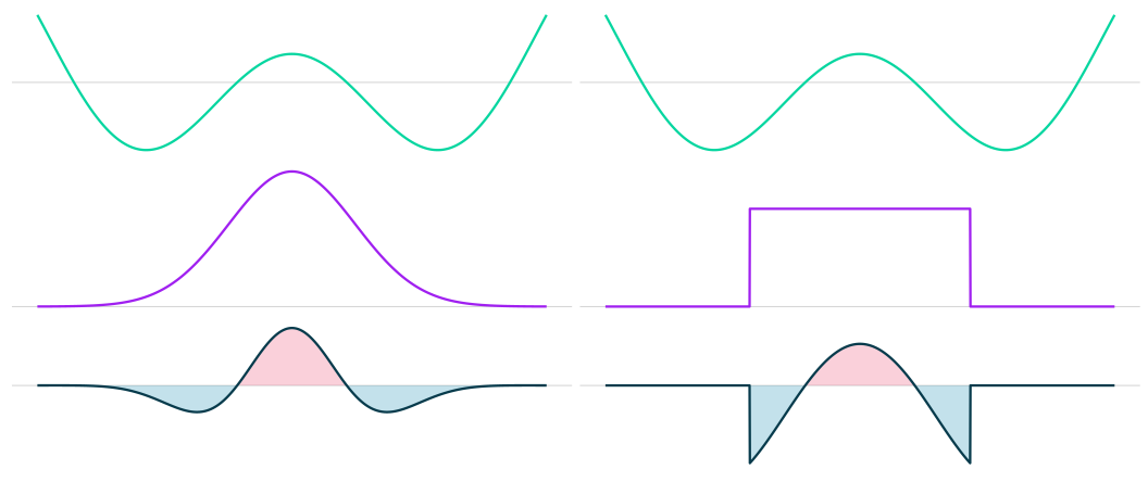
The normal satisfies this for every nice function u. \int \textcolor{#06D6A0}{\{u'(x)-xu(x)\}}\,\textcolor{#A020F0}{f_Z(x)}\,dx=0. Not every distribution does.

Only the normal has this signature

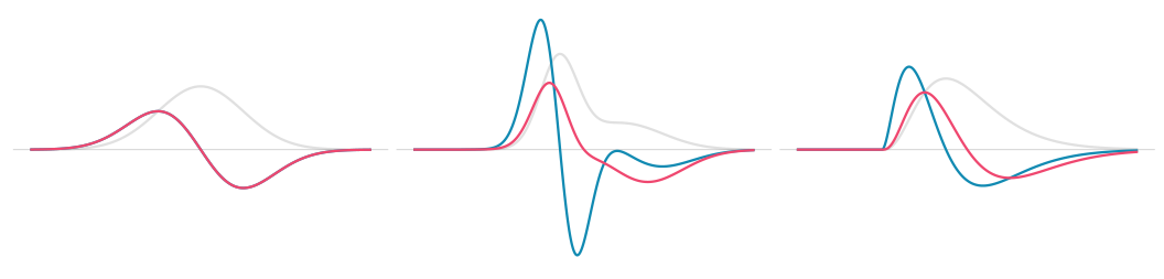
\begin{aligned} 0 &\overset{\mathtip{\small{\text{?}}}{\text{The defining signature is zero for every test function.}}}{=}\mathbb E\{u'(W)-Wu(W)\}\\ &\overset{\mathtip{\small{\text{?}}}{\text{Use linearity and write both expectations as density integrals.}}}{=}\int u'(x)f_W(x)\,dx-\int xu(x)f_W(x)\,dx\\ &\overset{\mathtip{\small{\text{?}}}{\text{Integrate the first term by parts; compact support of }u\text{ makes the boundary term zero.}}}{=}-\int u(x)f_W'(x)\,dx-\int xu(x)f_W(x)\,dx\\ &\overset{\mathtip{\small{\text{?}}}{\text{Factor }u(x)\text{ from the two integrands.}}}{=}-\int u(x)\{\textcolor{#118AB2}{f_W'(x)}+\textcolor{#EF476F}{xf_W(x)}\}\,dx. \end{aligned} Because this is zero for every u, the thing in brackets has to be zero.

-\int u(x)\{\textcolor{#118AB2}{f_W'(x)}+\textcolor{#EF476F}{xf_W(x)}\}\,dx=0\quad\text{for every }u\qquad\overset{\mathtip{\small{\text{?}}}{\begin{gathered} \text{Take }u(x)=\textcolor{#118AB2}{f_W'(x)}+\textcolor{#EF476F}{xf_W(x)}.\\ \text{Then the integral is }-\int\{\textcolor{#118AB2}{f_W'(x)}+\textcolor{#EF476F}{xf_W(x)}\}^2\,dx=0,\\ \text{so the bracket is zero. Smooth cutoffs justify this test when needed.} \end{gathered}}}{\iff}\textcolor{#118AB2}{f_W'(x)}+\textcolor{#EF476F}{xf_W(x)}=0.

That gives us a differential equation. And the normal density solves it. \textcolor{#118AB2}{f_W'(x)}\overset{\mathtip{\small{\text{?}}}{\text{Rearrange }f_W'(x)+xf_W(x)=0.}}{=}\textcolor{#EF476F}{-xf_W(x)} \qqtext{so} f_W(x)\overset{\mathtip{\small{\text{?}}}{\text{Solve the differential equation by separating variables and integrating.}}}{=}Ce^{-x^2/2} \qqtext{and} \int f_W\overset{\mathtip{\small{\text{?}}}{\text{A probability density has total integral one.}}}{=}1 \qqtext{gives} C\overset{\mathtip{\small{\text{?}}}{\text{Set the integral to one and solve for }C.}}{=}\frac1{\sqrt{2\pi}}.

Solving the signature equation

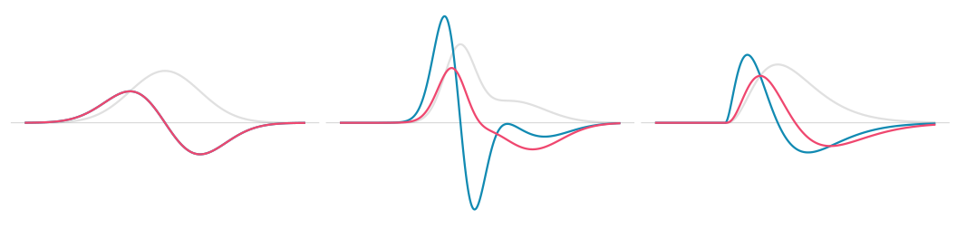
Divide by the density, and the left side is a derivative of a logarithm. \begin{aligned} \textcolor{#118AB2}{f_W'(x)}&=\textcolor{#EF476F}{-xf_W(x)}\\ \frac{f_W'(x)}{f_W(x)}&=-x\\ \{\log f_W(x)\}'&=-x\\ \log f_W(x)&=-\frac{x^2}{2}+c. \end{aligned}

How do we recover the density from its logarithm?

Exponentiate. The constant of integration becomes a factor, C=e^{c}. f_W(x)=Ce^{-x^2/2}. How do we find the constant?

A density integrates to one, which fixes it. \begin{aligned} C &= \frac{1}{\int_{-\infty}^{\infty}\exp(-x^2/2)\,dx}=\frac{1}{\sqrt{2\pi}}\\ f_W(x) &= C\exp(-x^2/2)=\frac{\exp(-x^2/2)}{\sqrt{2\pi}}. \end{aligned} This is the standard normal density.

Approximation: Sums almost have the normal signature

Here’s the phenomenon we’re going to explain

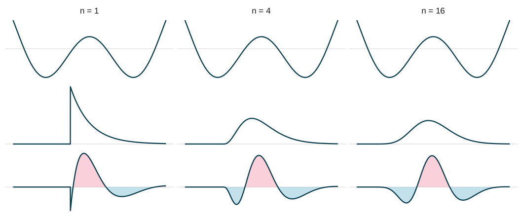
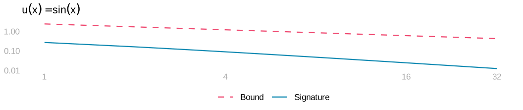
As we increase our sample size, shapes get more normal, and the signature gets smaller.

\left|\mathbb E\{u'(\textcolor{#073B4C}{W_n})-\textcolor{#073B4C}{W_n}u(\textcolor{#073B4C}{W_n})\}\right| \le\frac{M\mathbb E|Y_1-\mu|^3}{\sigma^3\sqrt n} \quad\text{when }|u''|\le M.

Now we’re gonna prove it.

Linearizing around Zero

The signature is the accumulated error of linearizing at zero change.
- We want to show this when the responses are independent.
- In each term, the change is \textcolor{#073B4C}{W}-\textcolor{#A020F0}{W_i'}. The calculation on the next slide will show this exactly.
It’ll help to make each term small. To do that, we’ll subtract zero. We just have to write it the right way.
Swapping one contribution for an independent copy gives us the zero we need.

\mathbb E\left\{\sum_i\textcolor{#073B4C}{X_i}u(\textcolor{#A020F0}{W_i'})\right\} \overset{\mathtip{\small{\text{?}}}{\begin{gathered}\textcolor{#073B4C}{X_i}\text{ is independent of }\textcolor{#A020F0}{W_i'}.\\\mathbb E\textcolor{#073B4C}{X_i}=0.\end{gathered}}}{=}\sum_i\underbrace{\mathbb E\textcolor{#073B4C}{X_i}}_{0} \,\mathbb E\{u(\textcolor{#A020F0}{W_i'})\}=0 \quad\text{where }\textcolor{#A020F0}{W_i'}=\textcolor{#073B4C}{W}-\textcolor{#073B4C}{X_i}+\textcolor{#EF476F}{X_i'}.
Subtracting this zero leaves small differences. Their linear part gives the other half of the signature.

\begin{aligned} \mathbb E\{\textcolor{#073B4C}{W}u(\textcolor{#073B4C}{W})\} &=\mathbb E\{\textcolor{#073B4C}{W}u(\textcolor{#073B4C}{W})\} -\underbrace{\mathbb E\left\{\sum_i\textcolor{#073B4C}{X_i}u(\textcolor{#A020F0}{W_i'})\right\}}_{0}\\ &=\sum_i\mathbb E\left[\textcolor{#073B4C}{X_i}\{u(\textcolor{#073B4C}{W})-u(\textcolor{#A020F0}{W_i'})\}\right]\\ &\approx\sum_i\mathbb E\{\textcolor{#073B4C}{X_i}(\textcolor{#073B4C}{W}-\textcolor{#A020F0}{W_i'})u'(\textcolor{#A020F0}{W_i'})\}. \end{aligned}
How good is this approximation? Here \tilde W_i lies between \textcolor{#A020F0}{W_i'} and \textcolor{#073B4C}{W}.

\begin{aligned} u(\textcolor{#073B4C}{W})-u(\textcolor{#A020F0}{W_i'}) &=(\textcolor{#073B4C}{W}-\textcolor{#A020F0}{W_i'})u'(\textcolor{#A020F0}{W_i'})\\ &\quad+\frac12u''(\tilde W_i)(\textcolor{#073B4C}{W}-\textcolor{#A020F0}{W_i'})^2. \end{aligned}

The calculation

The linear part averages to \mathbb E u'(\textcolor{#073B4C}{W}). Only the Taylor errors remain.

\begin{aligned} \mathbb E\{\textcolor{#073B4C}{W}u(\textcolor{#073B4C}{W})\} &\overset{\mathtip{\small{\text{?}}}{\text{Expand }\textcolor{#073B4C}{W}=\sum_i\textcolor{#073B4C}{X_i}\text{ and average the sum.}}}{=} \sum_i\mathbb E\{\textcolor{#073B4C}{X_i} u(\textcolor{#073B4C}{W})\}\\ &\overset{\mathtip{\small{\text{?}}}{\begin{gathered}\text{Subtract zero: independence and centering give}\\ \mathbb E\{\textcolor{#073B4C}{X_i} u(\textcolor{#A020F0}{W_i'})\}=\mathbb E \textcolor{#073B4C}{X_i}\,\mathbb E u(\textcolor{#A020F0}{W_i'})=0.\end{gathered}}}{=} \sum_i\mathbb E\left[\textcolor{#073B4C}{X_i}\{u(\textcolor{#073B4C}{W})-u(\textcolor{#A020F0}{W_i'})\}\right]\\ &\overset{\mathtip{\small{\text{?}}}{\begin{gathered}\text{Use the tangent at }\textcolor{#A020F0}{W_i'}:\\ u(\textcolor{#073B4C}{W})-u(\textcolor{#A020F0}{W_i'})\approx(\textcolor{#073B4C}{W}-\textcolor{#A020F0}{W_i'})u'(\textcolor{#A020F0}{W_i'}).\end{gathered}}}{\approx} \sum_i\mathbb E\{\textcolor{#073B4C}{X_i}(\textcolor{#073B4C}{W}-\textcolor{#A020F0}{W_i'})u'(\textcolor{#A020F0}{W_i'})\}\\ &\overset{\mathtip{\small{\text{?}}}{\textcolor{#073B4C}{W}-\textcolor{#A020F0}{W_i'}=\textcolor{#073B4C}{X_i}-\textcolor{#EF476F}{X_i'}.}}{=} \sum_i\mathbb E\{\textcolor{#073B4C}{X_i}(\textcolor{#073B4C}{X_i}-\textcolor{#EF476F}{X_i'})u'(\textcolor{#A020F0}{W_i'})\}\\ &\overset{\mathtip{\small{\text{?}}}{\text{Expand the product into two terms.}}}{=} \sum_i\left[\mathbb E\{\textcolor{#073B4C}{X_i}^2u'(\textcolor{#A020F0}{W_i'})\} -\mathbb E\{\textcolor{#073B4C}{X_i}\textcolor{#EF476F}{X_i'}u'(\textcolor{#A020F0}{W_i'})\}\right]\\ &\overset{\mathtip{\small{\text{?}}}{\textcolor{#073B4C}{X_i}\text{ is independent of the pair }(\textcolor{#EF476F}{X_i'},\textcolor{#A020F0}{W_i'}).}}{=} \sum_i\left[\mathbb E(\textcolor{#073B4C}{X_i}^2)\,\mathbb E u'(\textcolor{#A020F0}{W_i'}) -\mathbb E\textcolor{#073B4C}{X_i}\,\mathbb E\{\textcolor{#EF476F}{X_i'}u'(\textcolor{#A020F0}{W_i'})\}\right]\\ &\overset{\mathtip{\small{\text{?}}}{\mathbb E\textcolor{#073B4C}{X_i}=0.}}{=} \sum_i\mathbb E(\textcolor{#073B4C}{X_i}^2)\,\mathbb E u'(\textcolor{#A020F0}{W_i'})\\ &\overset{\mathtip{\small{\text{?}}}{\begin{gathered}\textcolor{#A020F0}{W_i'}\text{ and }\textcolor{#073B4C}{W}\text{ have the same distribution.}\\ \text{The same function has the same expectation:}\\ \mathbb E u'(\textcolor{#A020F0}{W_i'})=\mathbb E u'(\textcolor{#073B4C}{W}).\end{gathered}}}{=} \sum_i\mathbb E(\textcolor{#073B4C}{X_i}^2)\,\mathbb E u'(\textcolor{#073B4C}{W})\\ &\overset{\mathtip{\small{\text{?}}}{\text{The expectation of the same function of }\textcolor{#073B4C}{W}\text{ is common to every term.}}}{=} \left\{\sum_i\mathbb E(\textcolor{#073B4C}{X_i}^2)\right\}\mathbb E u'(\textcolor{#073B4C}{W})\\ &\overset{\mathtip{\small{\text{?}}}{\begin{gathered}\text{The centered contributions' variances sum to one:}\\ \sum_i\mathbb E(\textcolor{#073B4C}{X_i}^2)=1.\end{gathered}}}{=} \mathbb E u'(\textcolor{#073B4C}{W}). \end{aligned}

The signature is the error of this approximation. \mathbb E\{u'(\textcolor{#073B4C}{W})-\textcolor{#073B4C}{W}u(\textcolor{#073B4C}{W})\} =-\sum_i\mathbb E(\textcolor{#073B4C}{X_i}r_i) \qwhere r_i=u(\textcolor{#073B4C}{W})-u(\textcolor{#A020F0}{W_i'})-(\textcolor{#073B4C}{W}-\textcolor{#A020F0}{W_i'})u'(\textcolor{#A020F0}{W_i'}).

Bounding the remainder

One swap gives a quadratic remainder. Here \tilde W_i lies between \textcolor{#A020F0}{W_i'} and \textcolor{#073B4C}{W}.

\begin{aligned} r_i&=u(\textcolor{#073B4C}{W})-u(\textcolor{#A020F0}{W_i'}) -(\textcolor{#073B4C}{W}-\textcolor{#A020F0}{W_i'})u'(\textcolor{#A020F0}{W_i'})\\ &=\frac12u''(\tilde W_i)(\textcolor{#073B4C}{X_i}-\textcolor{#EF476F}{X_i'})^2 \quad\text{where }\textcolor{#073B4C}{W}-\textcolor{#A020F0}{W_i'}=\textcolor{#073B4C}{X_i}-\textcolor{#EF476F}{X_i'}. \\ |r_i|&\le\frac M2(\textcolor{#073B4C}{X_i}-\textcolor{#EF476F}{X_i'})^2 \quad\text{when }|u''|\le M. \end{aligned}

The signature weights each remainder by one contribution. That is why third moments appear.
- The swap tool bounds each term. Identical distributions then give the factor n/n^{3/2}.

\begin{aligned} \left|\mathbb E\{u'(\textcolor{#073B4C}{W})-\textcolor{#073B4C}{W}u(\textcolor{#073B4C}{W})\}\right| &\overset{\mathtip{\small{\text{?}}}{\text{Take absolute values inside the sum and expectation.}}}{\le}\sum_i\mathbb E|\textcolor{#073B4C}{X_i}r_i|\\ &\overset{\mathtip{\small{\text{?}}}{\text{Apply the Taylor error bound to each remainder.}}}{\le}\frac M2\sum_i\mathbb E\{|\textcolor{#073B4C}{X_i}|(\textcolor{#073B4C}{X_i}-\textcolor{#EF476F}{X_i'})^2\}\\ &\overset{\mathtip{\small{\text{?}}}{\begin{gathered}\text{Use the swap bound from Tools:}\\\mathbb E\{|\textcolor{#073B4C}{X_i}|(\textcolor{#073B4C}{X_i}-\textcolor{#EF476F}{X_i'})^2\}\le 2\mathbb E|\textcolor{#073B4C}{X_i}|^3.\end{gathered}}}{\le}M\sum_i\mathbb E|\textcolor{#073B4C}{X_i}|^3\\ &\overset{\mathtip{\small{\text{?}}}{\begin{gathered}\text{The contributions have identical distributions.}\\\textcolor{#073B4C}{X_i}=\textcolor{#073B4C}{(Y_i-\mu)/(\sigma\sqrt n)}.\end{gathered}}}{=}M\textcolor{#118AB2}{n}\, \mathbb E\left|\textcolor{#073B4C}{\frac{Y_1-\mu}{\sigma\sqrt n}}\right|^3\\ &\overset{\mathtip{\small{\text{?}}}{\text{Cube the scale factor }1/(\sigma\sqrt n).}}{=}M\frac{\textcolor{#118AB2}{n}}{n^{3/2}} \frac{\mathbb E|Y_1-\mu|^3}{\sigma^3}\\ &\overset{\mathtip{\small{\text{?}}}{n/n^{3/2}=1/\sqrt n.}}{=}\frac{M\mathbb E|Y_1-\mu|^3}{\sigma^3\sqrt n}. \end{aligned}

This bound tends to zero when the absolute third centered moment is finite. A larger third moment gives a larger bound.
- The sum-of-moments bound also applies to independent contributions with different distributions.

How does a small signature bound the distance from normal?

Continuity: If signatures are close, so are distributions

The bound

We measure distance by the largest difference between averages of functions with slope bounded by one.
- Such functions give nearby outcomes nearby values: |h(x)-h(y)|\le|x-y|.
- We’ll write this condition as |h'|\le1, allowing corners.

\textcolor{#118AB2}{d(W,Z)}=\max_{|h'|\le1} |\mathbb E h(W)-\mathbb E h(Z)|.

Why this distance? It’s continuous with respect to the signature.
- The distance goes to zero when the signature goes to zero uniformly.
- Uniformly means over all functions with curvature at most two.

\textcolor{#118AB2}{d(W,Z)}\le\textcolor{#EF476F}{\max_{|u''|\le 2} \left|\mathbb E\{u'(W)-Wu(W)\}\right|}.

It’s a pretty reasonable distance too. We’ll see.

Why it holds

We want to bound differences in averages. We have a bound on signatures.
- Wishful thinking: make each difference a signature.
For each \textcolor{#06D6A0}{h} with |h'|\le1, what would a matching \textcolor{#A020F0}{u_h} have to do?

\textcolor{#A020F0}{u_h'}(x)-x\textcolor{#A020F0}{u_h}(x)=\textcolor{#06D6A0}{h}(x)-\mathbb E\textcolor{#06D6A0}{h}(Z).
- Substitute W for x and average. The two sides are exactly the quantities we wanted to connect.
Solving gives us the match, with the curvature bound we need.

\textcolor{#A020F0}{u_h}(x)=\frac{1}{f_Z(x)} \int_{-\infty}^{x}\{\textcolor{#06D6A0}{h}(t)-\mathbb E\textcolor{#06D6A0}{h}(Z)\}f_Z(t)\,dt \quad\text{and}\quad |\textcolor{#A020F0}{u_h''}|\le2.
- We can check the solution by differentiating it.
- And we can get the curvature bound from the differential equation.
Now we can simplify: maximize over all functions with curvature at most two.
- Every match is included, so the maximum can only increase.
\begin{aligned} d(W,Z) &=\max_{|h'|\le1}\left|\mathbb E\{\textcolor{#A020F0}{u_h'}(W)-W\textcolor{#A020F0}{u_h}(W)\}\right|\\ &\le\max_{|u''|\le2}\left|\mathbb E\{u'(W)-Wu(W)\}\right|. \end{aligned}

Why this distance?

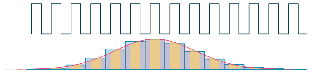
Bounded height doesn’t work.

There are functions with |h|\le1 that distinguish a discrete distribution from a continuous one.
- These spikes reach one at every possible outcome of W.
- Making them thinner leaves their average under W at one.
- Their average under the normal Z goes to zero.

\begin{aligned} \textcolor{#118AB2}{\mathbb E h(W)}&=\sum_w h(w)\mathbb P(W=w)=1,\\ \textcolor{#EF476F}{\mathbb E h(Z)}&=\int_{-\infty}^{\infty}h(x)f_Z(x)\,dx\longrightarrow0. \end{aligned}

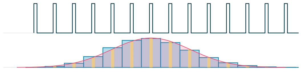
Bounded height doesn’t work.

There are functions with |h|\le1 that distinguish a discrete distribution from a continuous one.
- These spikes reach one at every possible outcome of W.
- Making them thinner leaves their average under W at one.
- Their average under the normal Z goes to zero.

\begin{aligned} \textcolor{#118AB2}{\mathbb E h(W)}&=\sum_w h(w)\mathbb P(W=w)=1,\\ \textcolor{#EF476F}{\mathbb E h(Z)}&=\int_{-\infty}^{\infty}h(x)f_Z(x)\,dx\longrightarrow0. \end{aligned}

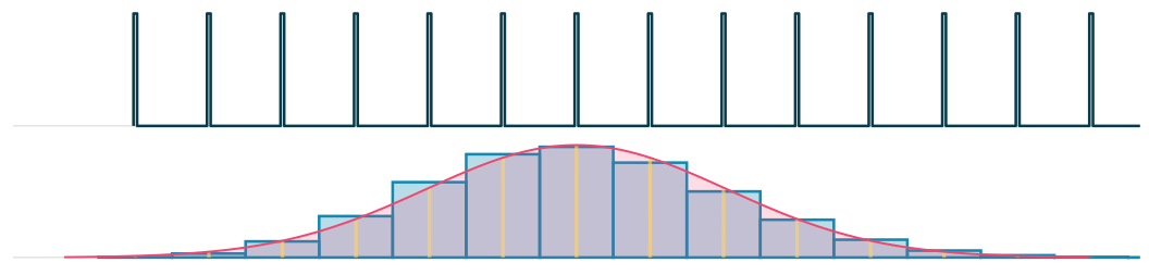
Bounded height doesn’t work.

There are functions with |h|\le1 that distinguish a discrete distribution from a continuous one.
- These spikes reach one at every possible outcome of W.
- Making them thinner leaves their average under W at one.
- Their average under the normal Z goes to zero.

\begin{aligned} \textcolor{#118AB2}{\mathbb E h(W)}&=\sum_w h(w)\mathbb P(W=w)=1,\\ \textcolor{#EF476F}{\mathbb E h(Z)}&=\int_{-\infty}^{\infty}h(x)f_Z(x)\,dx\longrightarrow0. \end{aligned}

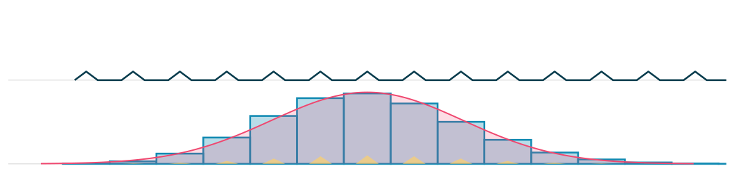
Bounded slope does work.

A function with bounded slope must give nearby outcomes nearby values.
- Even at the original width, the tents have to be shallow. Their averages under both W and Z are small.
A small move in outcomes changes the average of any allowed function only a little.
That lets a discrete distribution approach a continuous one in this distance.

|h'|\le1 \quad\Longrightarrow\quad \left|\frac{h(x)-h(y)}{x-y}\right|\le1.

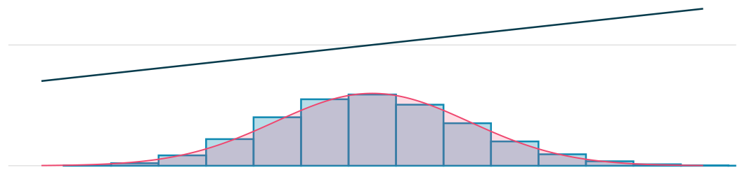
Bounded slope does work.

These functions give nearly the same average under W and Z.

\begin{aligned} h(x)&=x,\quad\text{with }|h'|\le1,\\ \textcolor{#118AB2}{\mathbb E h(W)}&\approx\textcolor{#EF476F}{\mathbb E h(Z)}. \end{aligned}

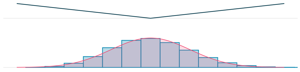
Bounded slope does work.

These functions give nearly the same average under W and Z.

\begin{aligned} h(x)&=|x|,\quad\text{with }|h'|\le1,\\ \textcolor{#118AB2}{\mathbb E h(W)}&\approx\textcolor{#EF476F}{\mathbb E h(Z)}. \end{aligned}

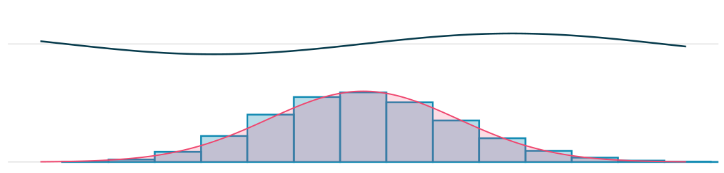
Bounded slope does work.

These functions give nearly the same average under W and Z.

\begin{aligned} h(x)&=\sin x,\quad\text{with }|h'|\le1,\\ \textcolor{#118AB2}{\mathbb E h(W)}&\approx\textcolor{#EF476F}{\mathbb E h(Z)}. \end{aligned}

Visualizing our distance

The distance is the area between the CDFs. We get this by integrating by parts.

\begin{aligned} d(W,Z) &=\max_{|h'|\le1}|\mathbb E h(W)-\mathbb E h(Z)|\\ &=\max_{|h'|\le1}\left|\int_{-\infty}^{\infty}h(x)\{\textcolor{#118ab2}{f_W(x)}-\textcolor{#ef476f}{f_Z(x)}\}\,dx\right|\\ &=\max_{|h'|\le1}\left|\int_{-\infty}^{\infty}h'(x)\{\textcolor{#ef476f}{F_Z(x)}-\textcolor{#118ab2}{F_W(x)}\}\,dx\right| \quad\text{where }\textcolor{#ef476f}{F_Z(x)}=\int_{-\infty}^{x}\textcolor{#ef476f}{f_Z(t)}\,dt\\ &=\left|\int_{-\infty}^{\infty}h'(x)\{\textcolor{#ef476f}{F_Z(x)}-\textcolor{#118ab2}{F_W(x)}\}\,dx\right| \quad\text{for }h'(x)=\begin{cases} +1&\text{if }\textcolor{#ef476f}{F_Z(x)}-\textcolor{#118ab2}{F_W(x)}\ge0,\\ -1&\text{if }\textcolor{#ef476f}{F_Z(x)}-\textcolor{#118ab2}{F_W(x)}<0 \end{cases}\\ &=\int_{-\infty}^{\infty}|\textcolor{#ef476f}{F_Z(x)}-\textcolor{#118ab2}{F_W(x)}|\,dx. \end{aligned}

We used densities here. This all works for distributions without densities—such as discrete distributions—but it requires a few extra steps or familiarity with some new ideas.

Summary

When Y_1\ldots Y_n are independent responses drawn from the same distribution, with mean \mu and variance \sigma^2, \small{ W_n=\frac{\sum_{i=1}^n(Y_i-\mu)}{\sigma\sqrt n}\quad\text{satisfies}\quad d(W_n,Z)\le\frac{2\mathbb E|Y_1-\mu|^3}{\sigma^3\sqrt n}\quad\text{where }d(W,Z)=\max_{|h'|\le1}|\mathbb E h(W)-\mathbb E h(Z)|. }

How did we prove it?

Characterization. Only the normal has zero signature for every test function. \mathbb E\{u'(W)-Wu(W)\}=0\ \text{ for every }u \quad\Longrightarrow\quad f_W'(x)=-xf_W(x) \quad\Longrightarrow\quad f_W(x)=\frac{e^{-x^2/2}}{\sqrt{2\pi}}.
Approximation. Sums have signatures close to zero. \left|\mathbb E\{u'(W_n)-W_nu(W_n)\}\right|\le \frac{M\mathbb E|Y_1-\mu|^3}{\sigma^3\sqrt n} \qquad\text{when }|u''|\le M.
Continuity. Close signatures mean close distributions. d(W_n,Z)\le\max_{|u''|\le2} \left|\mathbb E\{u'(W_n)-W_nu(W_n)\}\right|.