Normal Approximation and Sample Size Calculation

Review

$$ \newcommand{X}{} \newcommand{Y}{} % A hex digit after # inside a macro body is eaten by build-time expansion, so digit-leading hexes spell # via .

$$

Where We Left Off: Exact and Guaranteed

Sampling with replacement

Figure 1

Figure 2

Figure 3

Sampling without replacement

Figure 4

Figure 5

Figure 6

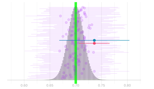
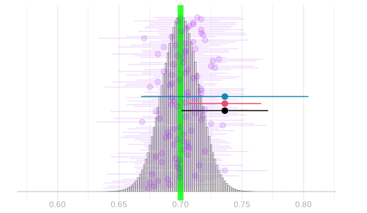
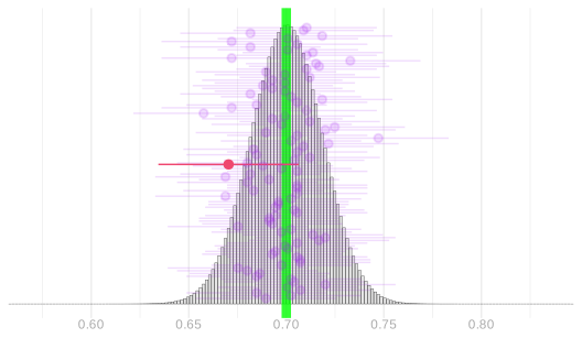
We now have three ways to calibrate an interval estimate.

1. Exact.
   • Needs the whole sampling distribution.
   • We have it for binary responses, sampled with or without replacement.
   • Outside that, a pain.
2. Chebyshev.
   • Needs only the standard deviation.
   • Conservative. Who wants to deny themselves precision that’s really there?
3. The bootstrap.
   • Works, often.
   • Not when sampling without replacement, unless n is tiny relative to m.
   • A thing you do, not a thing that helps you understand.

The Bootstrap

Figure 7

Figure 8

Figure 9

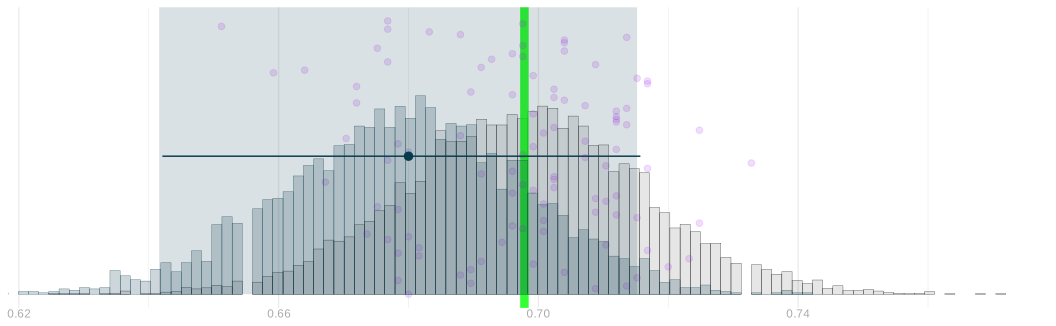
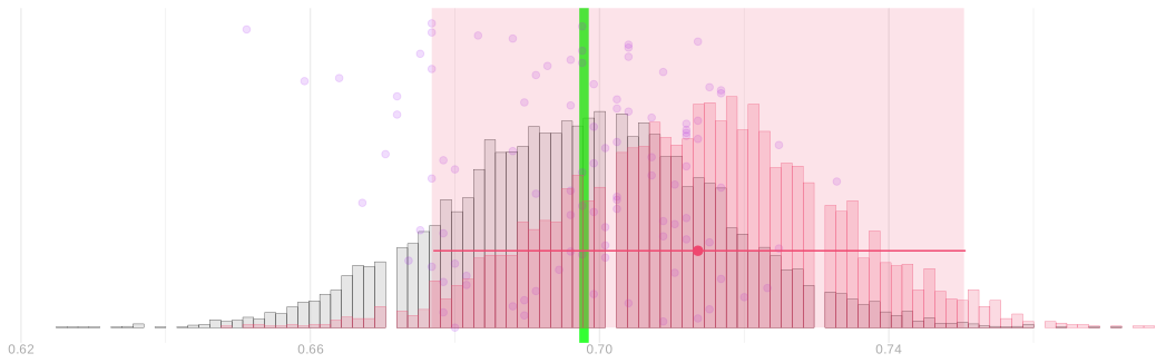
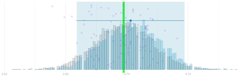
• The bootstrap. A general method for estimating sampling distributions.
  1. Draw a sample of size n from your sample. A bootstrap sample.
  2. Calculate your estimator on it. A bootstrap estimate.
  3. Repeat. The bootstrap sampling distribution.
• This simulates sampling with replacement.
  • Not sampling without. There’s no natural analog.
• Great for what we have learned after we have data.
  • Not for what we can learn before we have it.
• Today: a tool for that. Normal approximation.
  • And a job for it: sample size calculation. Choosing n so your interval is as narrow as you want.

Normal Approximation

The Normal Distribution

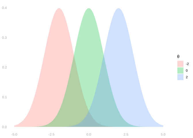
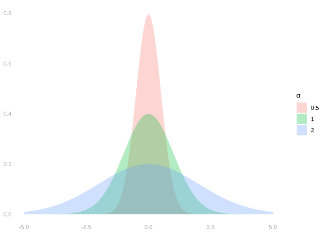
• The normal distribution is a parametric family of distributions involving two parameters.

  1. Its mean, \theta.
  2. Its standard deviation, \sigma.

• We say a random variable X is normally distributed with mean \theta and standard deviation \sigma …

• … if the probability that it’s in an interval [a,b] is given by this integral of its probability density. P_{\theta,\sigma}(X \in [a,b]) = \int_a^b f_{\theta,\sigma}(x)dx \qfor f_{\theta, \sigma}(x) = \frac{1}{\sqrt{2\pi}\sigma}e^{-\frac{(x-\theta)^2}{2\sigma^2}}

• We have to talk about the probability that it’s ‘in an interval’ rather than that it ‘takes a value’ because …

• … the probability it actually takes on any particular value is x zero: it’s an integral from x to x.

Normal Approximation

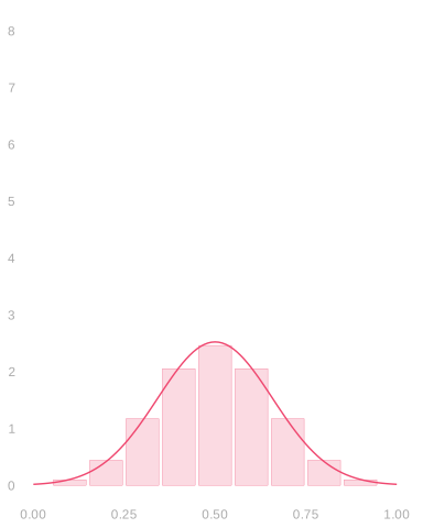
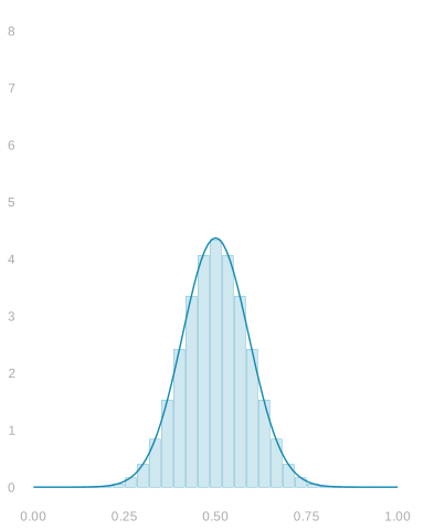
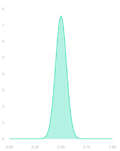
• A distribution’s normal approximation is a normal distribution with the same mean \theta and standard deviation \sigma.
  • These show up everywhere because they’re easy to work with and the approximation tends to be good.
  • Approximation is good, in particular, for the distribution of a mean of independent random variables.
  • Or independent enough ones.
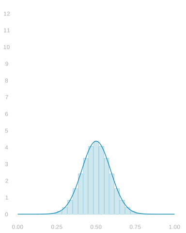
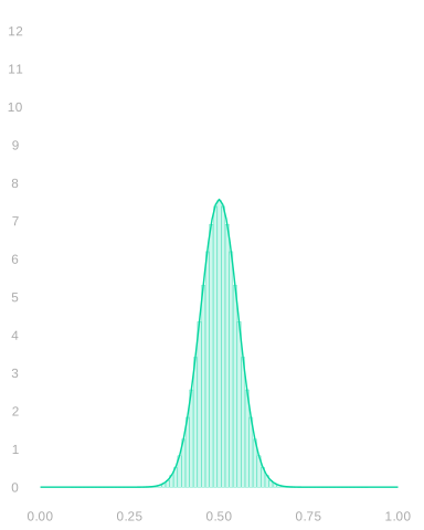
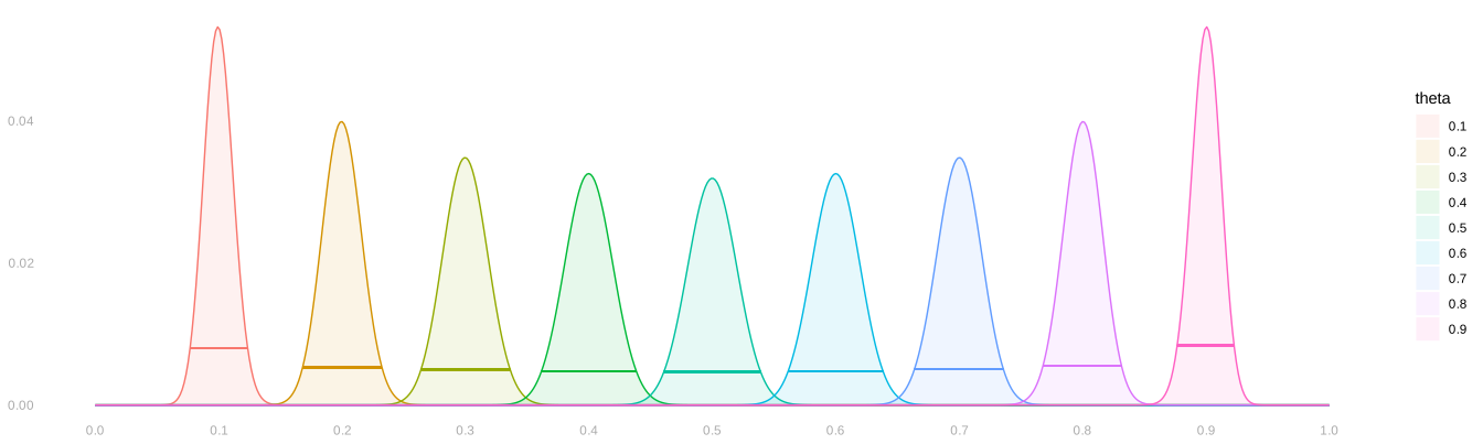
• Above, we see three Binomial distributions with their normal approximations:
  • the distributions of the mean of 10, 30, and 90 coin flips.
  • These approximations get increasingly accurate as the number of flips n increases.
  • That’s universal. It always happens with means. It’s called the Central Limit Theorem.

The Central Limit Theorem

The sampling distribution of a mean of independent random variables, \color{#404040}\frac{1}{n}\sum\limits_{i=1}^n X_i, gets arbitrarily close to its normal approximation
as the number of random variables \color{#404040}n increases to infinity.

Caveats.

• Finite variance. Without it, there is no normal limit.
• No single term dominates. Each one’s share of the mean’s variance has to be infinitesimal as \color{#404040}n \to \infty.
• Independence, or close to it. Dependence changes the variance, and enough of it changes the shape.

The Width of Normal Distributions

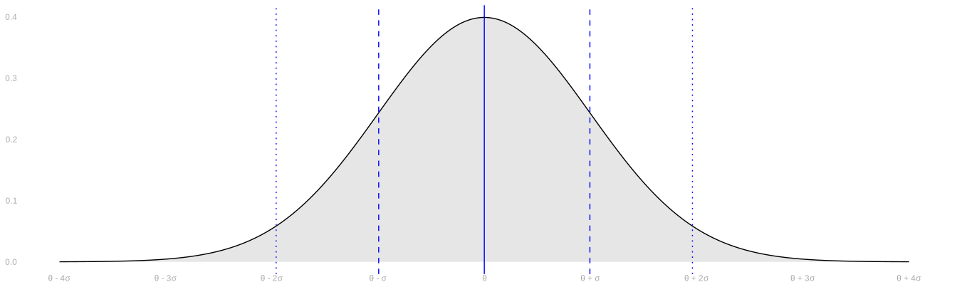
• One thing that’s convenient about the normal distribution is that it’s easy to reason about.
• In particular, it’s easy to reason about the width of its middle x%.
  • To include 68.3% of draws, you go out 1 standard deviation from its mean.
  • To include 95.4% of draws, you go out 2 standard deviations.
  • To include 99.7% of draws, you go out 3 standard deviations.
• To get almost exactly 95% of draws, we go out 1.96 standard deviations: \theta \pm 1.96\sigma.
  • Chebyshev got us 95% at \sqrt{20} \approx 4.5 standard deviations. The normal gets it at 1.96.
  • Same standard deviation. An interval 2.3\times narrower.
• Two is close enough in practice, but we tend to write 1.96 anyway.
  • It’s a signal about what we’re doing. You can get a 2 anywhere in a calculation.
  • When you see a 1.96, you know you’re talking about the middle 95% of the normal.

Calibration Using Normal Approximation

The (Binomial) sampling distribution and its normal approximation.

Binomial and normal estimates of the sampling distribution.

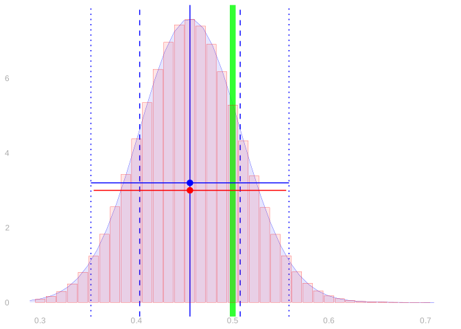
• Calibrating interval estimates using normal approximation is easy.
  • You estimate the standard deviation of your point estimator.
  • You go out ± 1.96 (estimated) standard deviations from your point estimate.

\text{interval estimate} = \hat\theta \pm 1.96 \hat\sigma

• We’re choosing our interval’s width essentially the same way we always have.
  • We’re still using the middle 95% of an estimate of the sample distribution.
  • It just looks different because we have a convenient formula for that width.
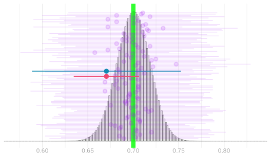
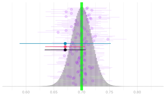
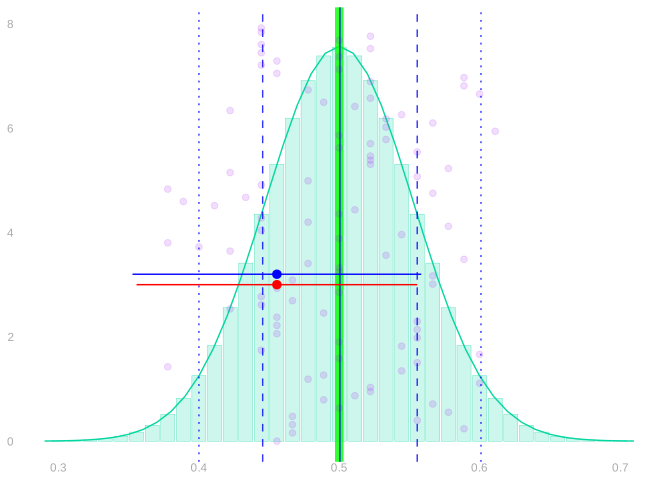
• Above left, you can see two interval estimates superimposed on the sampling distribution of a sample proportion.
  • The red one is calibrated using the binomial as before.
  • The blue one is calibrated using normal approximation.
• Above right, you can see the binomial and normal sampling distribution estimates these are based on.

When This Works

The (Binomial) sampling distribution and its normal approximation.

Binomial and normal estimates of the sampling distribution.

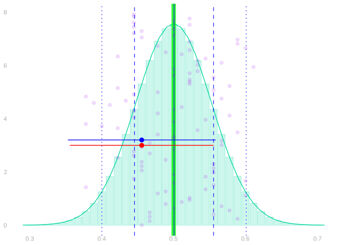
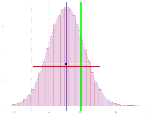
This works if three things are true.

1. The sampling distribution needs to be in the right place, i.e. centered on the estimation target.
   • This is called unbiasedness of our point estimator.
   • Most of the estimators we’ll talk about in this class are unbiased or almost unbiased.
2. The sampling distribution needs to be approximately normal.
   • The CLT tells us this tends to happen, especially for large n.
   • We’ll talk about how accurate it is next week. For most of the estimators we’ll study, you can take it as a given.
3. The estimated sampling distribution has approximately the right width.
   • This amounts to getting a good estimate of our point estimator’s standard deviation.
   • We’ll work on this, again for the sample proportion, later today. And for other estimators throughout the semester.
   • It is, however, a bit of a pain. That’s one reason you might prefer the bootstrap.

Normal Approximation in Context

A Proportion when Sampling with Replacement

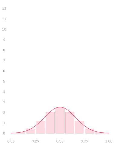
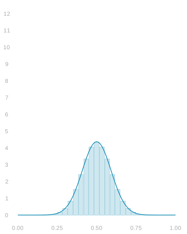
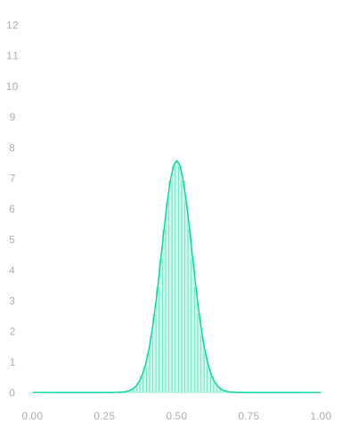
• When we sample from a binary population with replacement, our sample proportion’s distribution is Binomial.
  • And we can estimate that distribution by plugging our sample proportion into the Binomial formula.
  • But its normal approximation tends to be very good, so we can get away with estimating that instead.
  • Its standard deviation is the one we worked out last class.

\begin{aligned} \text{normal approximation} & \ f_{\theta,\sigma}(x) \qfor \sigma^2 = \frac{\theta(1-\theta)}{n} \\ \text{corresponding estimate} & \ f_{\hat\theta, \hat \sigma}(x) \qfor \hat\sigma^2 = \frac{\hat \theta(1-\hat \theta)}{n}. \end{aligned}

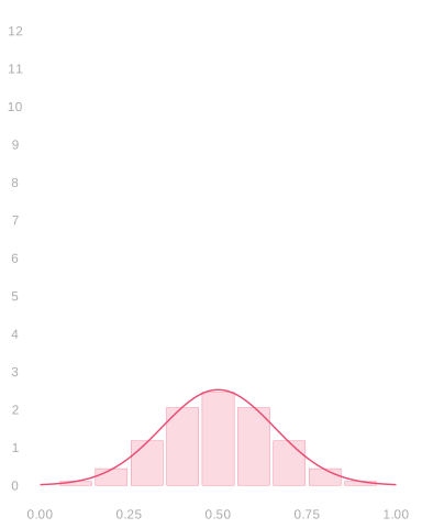
• Pictured: three Binomial distributions with their normal approximations.
  • These are the distributions of the sample proportion when we draw a samples of size 10, 30, and 90 …
  • … with replacement from a binary population in which the proportion of ones is \theta=.5.

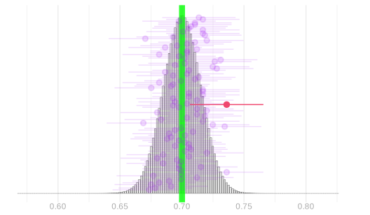
A Proportion when Sampling without Replacement

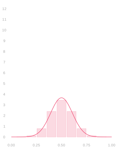
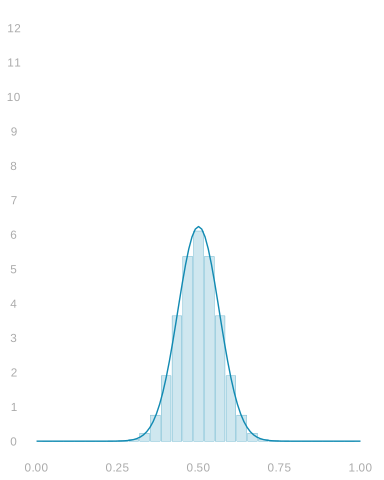
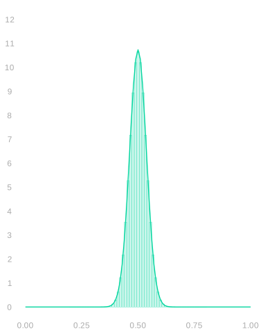
• Sampling without replacement from a binary population, our sample proportion is Hypergeometric.
  • We can estimate it by plugging our sample proportion into the Hypergeometric formula.
  • But again, its normal approximation is very good, so we can estimate that instead.
• This shows where we go wrong using the Binomial—or equivalently the bootstrap.
  • When \color{#404040}n is a meaningful fraction of \color{#404040}m, the Binomial is too wide.
  • Its standard deviation is the Binomial’s times \color{#404040}\sqrt{\frac{m-n}{m-1}}. A homework problem.
  • When we’re sampling half our population, i.e. n=m/2, that’s roughly \color{#404040}\sqrt{1/2} \approx .7.

\begin{aligned} \text{normal approximation} & \ f_{\theta,\sigma}(x) \qfor \sigma^2 = \frac{\theta(1-\theta)}{n} \times \frac{m-n}{m-1} \\ \text{corresponding estimate} & \ f_{\hat\theta, \hat \sigma}(x) \qfor \hat\sigma^2 = \frac{\hat \theta(1-\hat \theta)}{n} \times \frac{m-n}{m-1}. \end{aligned}

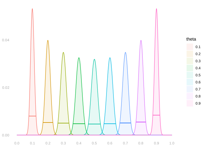
• Pictured: three Hypergeometric distributions with their normal approximations.
  • Sample proportions for samples of size 10, 30, and 90 …
  • … drawn without replacement from a binary population twice the size with \color{#404040}\theta=.5.

A Mean when Sampling with Replacement

Figure 10

Figure 11

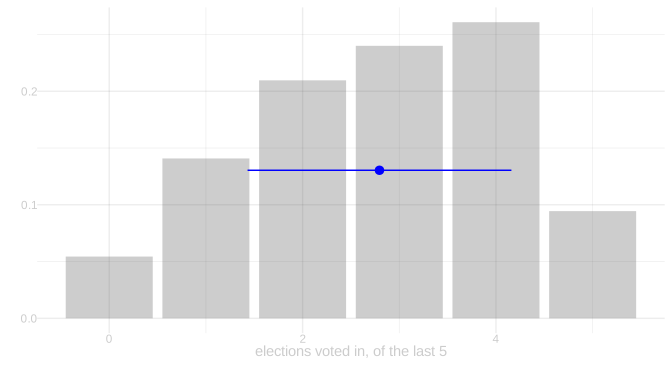
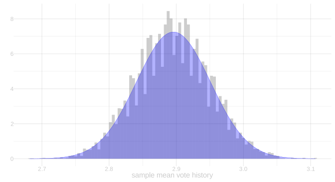
• Not special to proportions. Take the average vote history \bar H_n.
• Its standard deviation is the population standard deviation over \sqrt{n}. Plug in the sample’s.

\begin{aligned} \text{normal approximation} & \ f_{\mu,\sigma_n}(x) \qfor \sigma_n^2 = \frac{\sigma_H^2}{n} \qqtext{for} \sigma_H^2 = \frac{1}{m}\sum_{j=1}^m (h_j - \mu)^2 \\ \text{corresponding estimate} & \ f_{\bar H_n, \hat \sigma_n}(x) \qfor \hat\sigma_n^2 = \frac{\hat\sigma_H^2}{n} \qqtext{for} \hat\sigma_H^2 = \frac{1}{n}\sum_{i=1}^n (H_i - \bar H_n)^2. \end{aligned}

• Pictured: left, the 625 sampled voters’ vote histories with \bar H_n and the sample standard deviation.
  • Right, the sampling distribution of \bar H_n over draws from the population, with its normal approximation.

Using Normal Approximation

Figure 12

Figure 13

Figure 14

\begin{aligned} &f_{\hat\theta, \hat \sigma}(x) \qfor \hat\sigma^2 = \frac{\hat \theta(1-\hat \theta)}{n} && \text{a proportion when sampling with replacement} \\ &f_{\hat\theta, \hat \sigma}(x) \qfor \hat\sigma^2 = \frac{\hat \theta(1-\hat \theta)}{n} \times \frac{m-n}{m-1} && \text{a proportion when sampling without replacement} \\ &f_{\bar H_n, \hat \sigma_n}(x) \qfor \hat\sigma_n^2 = \frac{1}{n} \times \frac{1}{n}\sum_{i=1}^n (H_i - \bar H_n)^2 && \text{a mean when sampling with replacement} \end{aligned}

• What makes all this work is that we’re using good estimates of our estimator’s standard deviation.
  • If we have a formula for the estimator’s standard deviation, this is usuallly not so hard.
  • We estimate whatever population summaries show up in the formula and plug them in.

Sample Size Calculation

An Interval for Turnout in 2020

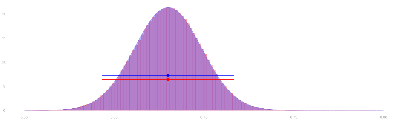
• Let’s compare our two approaches to calibration in our turnout poll.

\begin{aligned} \textcolor{red}{\text{binomial interval}} &= 0.6800 \pm 0.0368 \\ \textcolor{blue}{\text{normal interval}} &= 0.6800 \pm 0.0366 \end{aligned}

• We have to go out to 4 digits, way beyond what’s statistically meaningful, to see any difference in these intervals.
  • Our interval estimate—either one—is telling you might be off by a few hundredths.
  • Who cares about another couple ten-thousandths at the edge of the interval?

Thinking Speculatively About Intervals

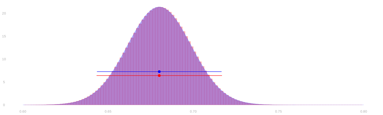
• Suppose we’re not satisfied with this level of precision, so we’re going to collect more data.
• Suppose we want our interval to be \pm .01 instead of \pm 0.037.
• How many people, in total, do we need to call? We can use the normal approximation to figure that out.

\hat \theta \pm 1.96\sigma_n \qfor \sigma_n = \sqrt{\frac{\theta (1-\theta)}{n}} \qqtext{ is } \hat\theta \pm .01 \qqtext{if} 1.96\sqrt{\frac{\theta (1-\theta)}{n}} = .01

• Now all we have to do is solve for n. And, since we don’t know \theta, use our best guess, \hat\theta=0.68.

n = \frac{1.96^2 \ \hat\theta (1-\hat\theta)}{.01^2} \approx 8000

The Easy Version

• There’s a trick to this. Let’s compare the interval width we have to the one we want.

\begin{aligned} \pm 0.037 &= \pm 1.96\hat\sigma_{625} \qfor \hat\sigma_{625} = \sqrt{\frac{\hat\theta (1-\hat\theta)}{625}} \\ \pm 0.01 &= \pm 1.96\hat\sigma_{n} \qfor \hat\sigma_{n} = \sqrt{\frac{\hat\theta (1-\hat\theta)}{n}} \end{aligned}

• All that changes in this formula is the sample size. And the sample size ratio falls out of the interval width ratio.

\frac{0.037}{.01} = \frac{1.96\hat\sigma_{625}}{1.96\hat\sigma_n} = \frac{\sqrt{\frac{\hat\theta (1-\hat\theta)}{625}}}{\sqrt{\frac{\hat\theta (1-\hat\theta)}{n}}} = \sqrt{\frac{n}{625}} \qqtext{ so } n = 625\left(\frac{0.037}{.01}\right)^2 \approx 8000

• To get the new sample size, multiply …
  • the sample size we have
  • the square of the desired ratio of the interval widths.
• To double precision, quadruple the sample size. To triple it, increase it 9x.
• To get another digit, i.e. increase precision 10x, increase the sample size 100x.

Starting from Scratch

Figure 15

• What do we do if we don’t have any data yet?

  • Then we don’t have a ‘current interval width’ to compare to the ‘desired interval width’.
  • And we don’t have a sample proportion \hat\theta to plug in for the population proportion \theta.

• But we can still use the formula we worked out earlier to get somewhere. 1.96\sqrt{\frac{\theta (1-\theta)}{n}} = .01 \qqtext{so} n = \frac{1.96^2 \ \theta (1-\theta)}{.01^2}

• We don’t have an estimate of \theta, but we do know it’s between 0 and 1. And, consequently, so is \theta(1-\theta).

• So we know that if we just substitute 1 into our formula, we’ll get a number that’s bigger than we need.

n < n' = \frac{1.96^2 \cdot 1}{.01^2} \approx 38400

• That’s a bit excessive. In fact, we can substitute in 1/4 instead of 1. n < n' = \frac{1.96^2 \cdot 1/4}{.01^2} \approx 9600

• Much better. That’s pretty close to the number we got with preliminary data.

Why Can We Use 1/4?

Figure 16

Figure 17

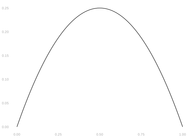
• Here’s the claim. Why is it true? n := \frac{1.96^2 \ \theta (1-\theta)}{.01^2} < n' := \frac{1.96^2 \ \times 1/4}{.01^2}

• Hint. Look at the graph of f(x) = x(1-x) above.

• Because 1/4 is the biggest \theta (1-\theta) gets for \theta \in [0,1].
• And it happens, for what it’s worth, when \theta = 1/2.
• That is, we’ll have the least precision — at a given sample size — when the proportion we’re estimating is 1/2.

Case Study

The NSW Experiment

The National Supported Work Demonstration

Figure 18

Figure 19

n	\hat \mu	sample SD
185	6300	7900

• The Program
• The Result

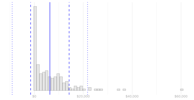
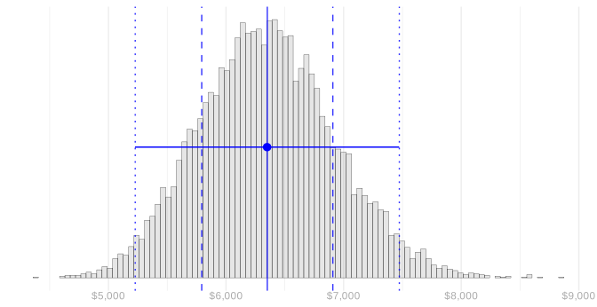
• The National Supported Work Demonstration was an experimental program in the 1970s that provided job training and other services.
• Here ‘experimental’ doesn’t just mean untested. It was run as a big experiment.
• From a population of eligible people, they drew a sample of size 445 to participate.
• To help estimate the impact of the program, participants were randomized into two groups.
  • The ‘treated’ group received the training and services.
  • The ‘control’ group did not.
• Today we’ll look at the treated group only: 185 people.

• A year or two after the program ended, they looked at the incomes of the people who’d been treated.
  • The average within the sample was about $6300 per year. In 1978 dollars.
  • A dollar in 1978 was worth about what $5 is today.
  • So adjusting for inflation, that’s an in-sample average of about $31700.
• But the sample was relatively small. And, as a result, the interval estimate is pretty wide.

\begin{aligned} \mu &\in 6300 \pm 1100 \approx [5200, \ 7500] &&\qqtext{is a 95\% confidence interval in 1978 dollars} \\ &\in 31700 \pm 5600 \approx [26100, \ 37400] &&\qqtext{adjusted for inflation} \end{aligned}

Activities

Figure 20

Figure 21

n	\hat \mu	sample SD
185	6300	7900

• Warm-Up
• Resizing

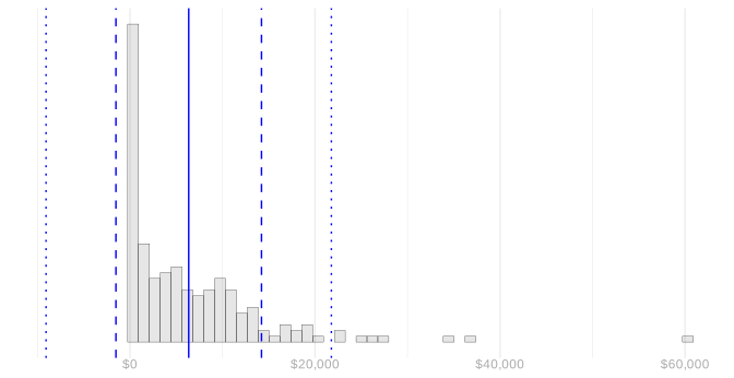
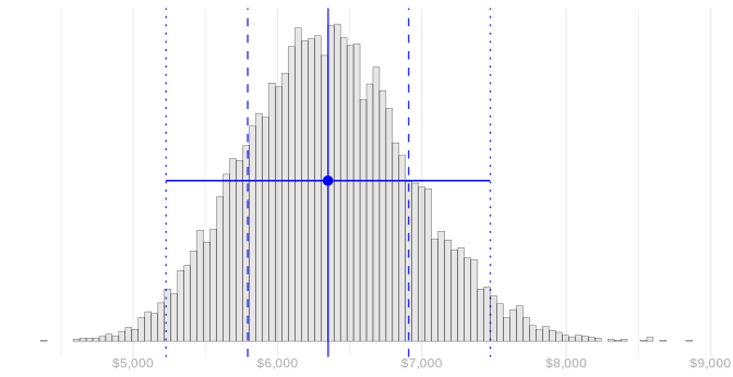
• Use the information in this table and the formulas to calculate a 95% interval based on normal approximation.
• Compare it to the interval we got using the bootstrap sampling distribution for calibration.

• Suppose we want to know the population mean to within $500 (1978 dollars).
• How can we resize our study to make that happen?
• We could run a second wave, drawing more people from the same population exactly as before, to get a larger sample like the one we have.
• What sample size would we need to be able to get a 95% confidence interval this accurate?

Solutions and Discussion

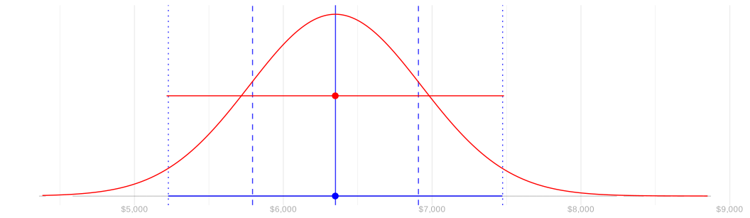
Figure 22

• Warm-Up. \hat\mu \pm 1.96\,\hat\sigma_n, with \hat\sigma_n the sample standard deviation over \sqrt{n}.
  • 6300 \pm 1.96 \times 7900/\sqrt{185} \approx 6300 \pm 1100. The bootstrap gave \pm 1100.

• Resizing, the hard way. Just like the turnout poll: we want \pm 500 instead of \pm 1130.

\hat\mu \pm 1.96\hat\sigma_n \qfor \hat\sigma_n = \frac{\hat\sigma_Y}{\sqrt{n}} \qqtext{ is } \hat\mu \pm 500 \qqtext{if} 1.96\frac{\hat\sigma_Y}{\sqrt{n}} = 500

• Now all we have to do is solve for n, using the sample standard deviation \hat\sigma_Y = 7900.

n = \frac{1.96^2 \ \hat\sigma_Y^2}{500^2} \approx 950

• Resizing, the easy way. Compare the interval width we have to the one we want.

\begin{aligned} \pm 1130 &= \pm 1.96\hat\sigma_{185} \qfor \hat\sigma_{185} = \frac{\hat\sigma_Y}{\sqrt{185}} \\ \pm 500 &= \pm 1.96\hat\sigma_n \qfor \hat\sigma_n = \frac{\hat\sigma_Y}{\sqrt{n}} \end{aligned}

• All that changes is the sample size. The sample size ratio falls out of the interval width ratio.

\frac{1130}{500} = \frac{1.96\hat\sigma_{185}}{1.96\hat\sigma_n} = \sqrt{\frac{n}{185}} \qqtext{ so } n = 185\left(\frac{1130}{500}\right)^2 \approx 950