7 Calibrating Interval Estimates with Binary Observations
Calibration
What does it mean for an interval estimate to be calibrated? We’ll work through a polling example to see why calibration matters and what goes wrong when you get it wrong.
Before the Election
$$ \newcommand{X}{} \newcommand{Y}{}
$$
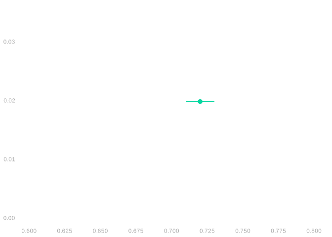
Before the election. You want to estimate the proportion of all registered voters—the population—who will vote. To do this, you use the proportion of polled voters—your sample—who said they would. You’re probably not going to match the population proportion exactly, so you report an interval estimate—a range of values we claim the population proportion is in. You know you’re not going to be right 100% of the time you make claims like this, so you state a nominal coverage probability—how often you’re right about claims like this.1
Without thinking too hard about it, you report, as your interval, your sample proportion (72%) ± 1%. Because it sounds good. And you say your coverage probability is 95%. Because that’s what everybody else says.
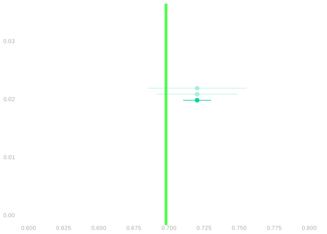
After the election. When the election occurs, we get to see who turns out to vote. 5.05M people, or roughly 70% of registered voters, actually vote. You—and future employers—can see how well you did. And how well everybody else did.
Your interval missed the target. It doesn’t contain the turnout proportion. Your point estimate is only off by 2%. But you overstated your precision. Now you’re kicking yourself. You’d briefly considered saying ± 3% or ± 4%. That would’ve done it. But that didn’t sound as good, so you went for ± 1%.
You hope you’re not the only one who missed. So you check out the competition.
The Competition
\[ \begin{array}{r|rr|rr|r|rr|r} \text{call} & 1 & & 2 & & \dots & 625 & & \\ \text{poll} & J_1 & Y_1 & J_2 & Y_2 & \dots & J_{625} & Y_{625} & \overline{Y}_{625} \\ \hline \color{\]
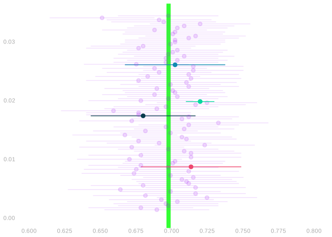
It turns out that everyone got their point estimate exactly like you did. Each of them rolled their 7.23M-sided die 625 times. And after making their 625 calls, they reported their sample proportion.
You’re not the only one who missed, but you’re part of a pretty small club. 5% of the other polls got it wrong. But you are the only one who claimed they’d get within 1%. Everyone else claimed they’d get within roughly 4%. Most were right. About 95%. And a lot of them had worse point estimates than you.
What you have is a calibration problem.
Calibration using the Sampling Distribution
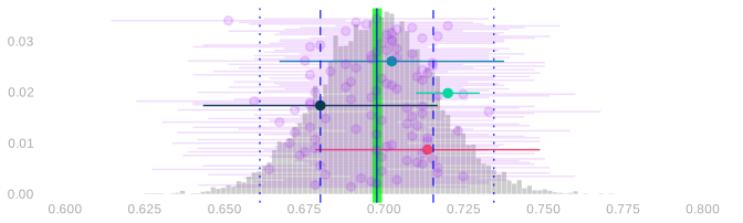
You’d have seen that your interval was miscalibrated if you knew what you do now: your competitors’ point estimates, which they got exactly like you got yours, and who actually turned out, so you could simulate even more polls if you wanted to.
You’d have drawn ± 1% intervals around all these point estimates.2 And noticed that many but not most of these intervals cover the target. About 43% do. Or, if leaving the target out of it, that only 43% of them cover the mean of all these estimates. Same thing. The mean and target are right on top of one another. Like this: |.
And you’d have known how to choose the right interval width. One that makes 95% of these intervals cover. Right?
Question
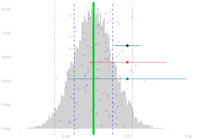
I’ve drawn the sampling distribution of an estimator, 100 draws from it as ●s, and 3 interval estimates. One of these interval estimates is calibrated to have exactly 95% coverage. Which is it?
- A. The one around the ● on top.
- B. The one around the ● in the middle.
- C. The one around the ● on the bottom.
Hint. You can reach your twin with your arms if your twin can reach you with theirs.
Hint. Maybe you look like this ● and your twin like this |.
Calibration in Reality
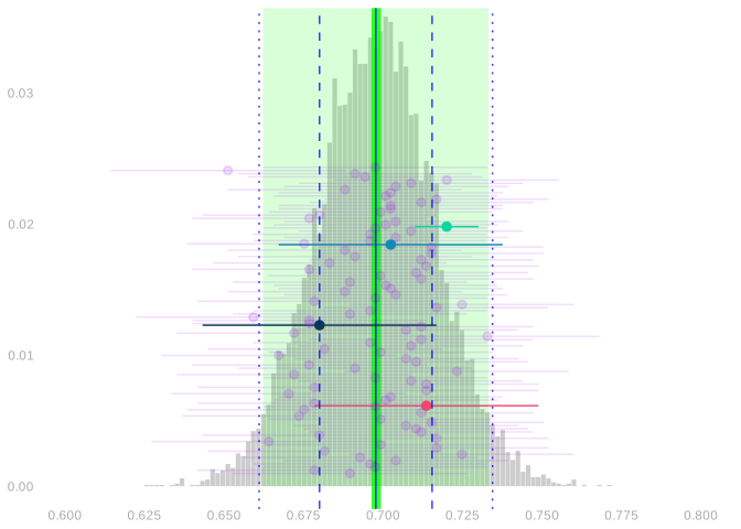
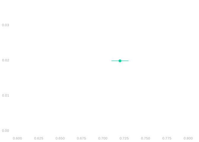
But you didn’t know any of this. You just knew your own point estimate. Without all that post-election information, you didn’t know how to calibrate an interval estimate. But everyone else did. Their widths were almost the same as the width you’d choose now.
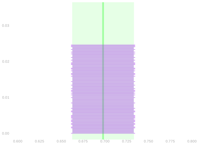
They didn’t know the point estimator’s actual sampling distribution, but they knew enough about it to choose the right interval width. That’s what we’re going to look into now. Over the course of this lecture and the next, we’ll work out what the sampling distributon of our estimator can look like and how what it does look like depends on the population. And we’ll see how to use that information to calibrate our intervals.