10  Sampling without Replacement and the Hypergeometric Distribution

$$ \newcommand{X}{} \newcommand{Y}{}

$$

Review: Sampling with Replacement

We calculated a sampling distribution last time, and we did it in two stages. First we went from calls to responses. Then we went from responses to their sum.

Think back to three calls to ten voters, with replacement. There were \(m_1\) Yes-voters and \(m_0\) No-voters, with \(m_1+m_0=10\). Each call could reach any of the ten people, including someone we’d already called.

Each of the eight things you could hear has three counts multiplied together underneath it, one per call, for the same reason as before — and \(10 \times 10 \times 10 = 10^3\) roll sequences in all.

Partially Marginalized

\(p\)	\(Y_1\)	\(Y_2\)	\(Y_3\)	\(Y_1+Y_2+Y_3\)
\(\frac{m_0^3}{10^3}\)	\(0\)	\(0\)	\(0\)	\(0\)
\(\frac{m_0^2 m_1}{10^3}\)	\(0\)	\(0\)	\(1\)	\(1\)
\(\frac{m_0^2 m_1}{10^3}\)	\(0\)	\(1\)	\(0\)	\(1\)
\(\frac{m_0^2 m_1}{10^3}\)	\(1\)	\(0\)	\(0\)	\(1\)
\(\frac{m_0 m_1^2}{10^3}\)	\(0\)	\(1\)	\(1\)	\(2\)
\(\frac{m_0 m_1^2}{10^3}\)	\(1\)	\(0\)	\(1\)	\(2\)
\(\frac{m_0 m_1^2}{10^3}\)	\(1\)	\(1\)	\(0\)	\(2\)
\(\frac{m_1^3}{10^3}\)	\(1\)	\(1\)	\(1\)	\(3\)

Fully Marginalized

\(p\)	\(Y_1+Y_2+Y_3\)
\(\frac{m_0^3}{10^3}\)	\(0\)
\(\frac{3 m_0^2 m_1}{10^3}\)	\(1\)
\(\frac{3 m_0 m_1^2}{10^3}\)	\(2\)
\(\frac{m_1^3}{10^3}\)	\(3\)

The left-hand column of the second table carries the multipliers \(1, 3, 3, 1\).

The first table has a row for each thing we could hear. The second table combines rows with the same sum. The three rows with one Yes have the same probability because moving the Yes only rearranges the factors of \(m_0^2m_1\).

Look at the cards you’ve laid out, with red for 1 and black for 0. If you don’t have cards, you’ll have to imagine them.

Understanding partial marginalization. Swap a card for another of the same colour. You called somebody else and you heard the same thing. The row doesn’t move; you’ve found another roll sequence sitting underneath it, and counting those is what the first stage does.

Understanding full marginalization. Move the cards you have into a different order. Now you’ve got a different row — a different thing to hear — with the same number of Yeses in it, so it lands on the same sum. Counting those is what the second stage does.

For \(n\) calls with replacement to \(m=m_1+m_0\) people, we wrote the population frequencies as \(\theta_1=m_1/m\) and \(\theta_0=m_0/m\). A response sequence \(a_1,\ldots,a_n\) is a binary sequence of length \(n\). If its sum is \(k\), the same two steps are

\[ \begin{aligned} P(Y_1=a_1,\ldots,Y_n=a_n)&=\theta_1^k\theta_0^{n-k},\\ P(Y_1+\ldots+Y_n=k)&=\binom{n}{k}\theta_1^k\theta_0^{n-k}. \end{aligned} \]

The first line has one factor for each response: \(k\) ones and \(n-k\) zeros. For the second, we sum the probabilities of all binary sequences with sum \(k\). With replacement, those sequences all have the same probability: rearranging the responses only rearranges the factors. So summing is counting and multiplying.

You could work out how to count binary sequences of length \(n\) with sum \(k\). But we talked about its name last class: the binomial coefficient, written \(\binom{n}{k}\) and read ‘\(n\) choose \(k\)’. You don’t need to derive the count to write the formula.

Check with R

In these cells, theta is \(\theta_1\), and x is the number of Yeses, which we called \(k\) above. Edit the inputs to check your calculation. x can be one value or a vector of values; 0:n checks them all.

Both steps were counting and multiplying: the call sequences were equally likely, and response sequences with the same sum had the same probability.

Now we sample without replacement: we can’t call the same person twice.

Which step changes? What stays the same? Think about it.

Sampling without Replacement: Two Exercises

The probability column in the first table changes. The second step stays the same: combine rows with the same number of Yeses. Those sequences still have equal probabilities, so we can still count them and multiply.

With that in mind, work through the two exercises below.

Three Calls from Ten People

Deal three cards from your ten without putting any back, and count the Yeses. That count has a distribution, and the distribution has a name: this is the hypergeometric distribution. Find its probabilities in the first exercise, then generalize to any number of calls.

ExerciseThree Calls

Ten voters: seven will vote and three won’t. Make three calls without replacement. Find the distribution of \(Y_1+Y_2+Y_3\).

Look at the ten cards you’ve laid out, Ace through 10: red is 1 and black is 0. These cards are our population. If you don’t have cards, you’ll have to imagine them. The example here uses seven red and three black; use your group’s own counts if they’re different. Draw three cards without putting them back.

1. Write the eight response sequences and calculate their probabilities.
2. Combine the sequences with the same sum.

To help count, lay out a response sequence such as red, red, black. Count the choices for each card as you take it from the population. Try rearranging the same colours and count again.

Checkpoint. Set m to your group’s number of cards and theta to the fraction that are red in the cell below. Check your numbers, then discuss your calculation with me before generalizing. Why do sequences with the same number of Yeses have the same probability?

Use the same inputs as in the review. Choose m and theta so that m * theta is a whole number of voters, and keep n no larger than m. The cell converts the population proportion into the two counts that dhyper needs.

SolutionThree Calls: Solution

There are \(10\times9\times8=720\) equally likely call sequences. Take ‘Yes,Yes,No’. There are seven choices for the first Yes, six for the second, and three for the No. That’s \(7\times6\times3=126\) call sequences that sound the same, so this response sequence has probability \(126/720\).

The tables have the same columns as before. What changes is the probability column: using a person up leaves one fewer choice the next time we need that response.

Partially Marginalized

\(p\)	\(Y_1\)	\(Y_2\)	\(Y_3\)	\(Y_1+Y_2+Y_3\)
\(\frac{3\times2\times1}{720}\)	\(0\)	\(0\)	\(0\)	\(0\)
\(\frac{3\times2\times7}{720}\)	\(0\)	\(0\)	\(1\)	\(1\)
\(\frac{3\times7\times2}{720}\)	\(0\)	\(1\)	\(0\)	\(1\)
\(\frac{7\times3\times2}{720}\)	\(1\)	\(0\)	\(0\)	\(1\)
\(\frac{3\times7\times6}{720}\)	\(0\)	\(1\)	\(1\)	\(2\)
\(\frac{7\times3\times6}{720}\)	\(1\)	\(0\)	\(1\)	\(2\)
\(\frac{7\times6\times3}{720}\)	\(1\)	\(1\)	\(0\)	\(2\)
\(\frac{7\times6\times5}{720}\)	\(1\)	\(1\)	\(1\)	\(3\)

Fully Marginalized

\(p\)	\(Y_1+Y_2+Y_3\)
\(\frac{6}{720}\)	\(0\)
\(\frac{3\times42}{720}\)	\(1\)
\(\frac{3\times126}{720}\)	\(2\)
\(\frac{210}{720}\)	\(3\)

Look at the three rows with two Yeses. Their numerators are \(3\times7\times6\), \(7\times3\times6\), and \(7\times6\times3\). Moving the No changes the order of the factors, not their product. So the second step is still counting and multiplying:

\[ P(Y_1+Y_2+Y_3=2) =\frac{126}{720}+\frac{126}{720}+\frac{126}{720} =3\times\frac{126}{720}. \]

The multipliers are still \(1,3,3,1\). The probability of each response sequence changed; the number of response sequences with each sum did not.

Generalize Your Answer

Exercise\(n\) Calls

Now \(n\) calls to \(m\) voters, of whom \(m_1\) will vote and \(m_0\) won’t, still without replacement. Find the distribution of \(Y_1 + \ldots + Y_n\).

Generalize your three-call calculation. Replace your population counts by \(m_1\) and \(m_0\), and replace three calls by \(n\) calls. Keep the same two steps: calls to responses, then responses to their sum.

For a response sequence with \(s\) Yeses, which factors appear in its probability? How many response sequences have that sum?

You won’t write out an arbitrarily large table. Spot-check a few rows: choose a response sequence and count the call sequences underneath it, then compare with your formula.

Check your formula by putting the three-call numbers back in. You can’t check arbitrary \(m\) and \(n\) computationally in the abstract, but you can try a couple of pairs. For each pair, choose how many of the \(m\) voters will vote, set m, n, and theta in the cell above, and compare its probabilities with your formula.

TipHint

Stage 2 you already have. Rows with the same sum still carry the same probability — the falling factor moves to a different call and the product doesn’t notice — so the count of rows is the one you counted last time.

Stage 1 is the one to redo, and the thing to work out is what each call uses up. When you’ve already heard three Yeses, how many Yeses are left to hear — and how many Nos?

SolutionGeneralization: Solution

To find the distribution of a sum \(Y_1 + \ldots + Y_n\) when we sample without replacement we do the same thing. We start by writing out the joint distribution of \(n\) calls. We’re equally likely to pull any sequence of \(n\) distinct numbers in \(1\ldots m\). There are \(m \times (m-1) \times \ldots \times (m-n+1)\) sequences, so the probability is \(1/\bigl[m(m-1)\ldots(m-n+1)\bigr]\) for each sequence. Then we add the responses and sums as columns. That doesn’t change.

Then we marginalize in two steps.

1. Sum over roll sequences leading to the same response sequence \(a_1 \ldots a_n\).
2. Sum over response sequences leading to the same sum \(s=a_1+\ldots+a_n\).

Step 1. Partial Marginalization

Here’s the partially marginalized table again. Each row represents a response sequence, and its last column is the number of Yeses. A row has probability zero if it asks for more of either response than the population contains.

Partially Marginalized

\(p\)	\(Y_1\)	\(Y_2\)	\(\ldots\)	\(Y_n\)	\(Y_1+\ldots+Y_n\)
\(\frac{m_0(m_0-1)\ldots(m_0-n+1)}{m(m-1)\ldots(m-n+1)}\)	\(0\)	\(0\)	\(\ldots\)	\(0\)	\(0\)
\(\frac{m_1\,m_0(m_0-1)\ldots(m_0-n+2)}{m(m-1)\ldots(m-n+1)}\)	\(0\)	\(0\)	\(\ldots\)	\(1\)	\(1\)
⋮	⋮	⋮	⋱	⋮	⋮
\(\frac{m_0\,m_1(m_1-1)\ldots(m_1-n+2)}{m(m-1)\ldots(m-n+1)}\)	\(1\)	\(1\)	\(\ldots\)	\(0\)	\(n-1\)
\(\frac{m_1(m_1-1)\ldots(m_1-n+1)}{m(m-1)\ldots(m-n+1)}\)	\(1\)	\(1\)	\(\ldots\)	\(1\)	\(n\)

There are still \(2^n\) response sequences. To fill the probability column, we count the distinct-person call sequences under each one. Each product has one factor per response of that kind; when there are none, that product is 1.

To sum over roll sequences, we sum over one roll after another. Suppose we’re calculating the probability of the response sequence \(a_1 \ldots a_n = 0,0,...,0,0\). First assume \(n\leq m_0\), so this sequence is possible.

1. We consider any ‘head’ \(j_1\ldots j_{n-1}\) where \(y_{j_1} \ldots y_{j_{n-1}}=0,0,...0\) and think about choosing the last element. No matter what the head is, we’ve ‘used up’ \(n-1\) people with response \(y_j=0\). So there are \(m_0-(n-1)=m_0-n+1\) ways to complete the sequence by choosing an as-yet unused \(j_{n}\) with \(y_{j_n}=0\).
2. We repeat with shortened ‘head’ \(j_1 \ldots j_{n-2}\) to consider the choice of \(j_{n-1}\). We have \(m_0-n+2\) as-yet unused choices and our last step tells us that each choice results in \(m_0-(n-1)\) call sequences, so there are \((m_0 - n + 1)(m_0 - n + 2)\) sequences with head \(j_1 \ldots j_{n-2}\) ending in \(0,0\).
3. Repeat \(n-2\) more times. We get \((m_0 - n + 1) \times \ldots \times m_0\) rows.

When we work through the same argument for sequences with a mix of 0s and 1s, we see that a call in the head forecloses possibilities for later calls with the same response only. Thus, when we have \(s\) ones and \(n-s\) zeros, we can think of ourselves as choosing calls with response zero and response one separately. We have \(\bigl[m_0(m_0-1)\ldots(m_0-(n-s)+1)\bigr]\times\bigl[m_1(m_1-1)\ldots(m_1-s+1)\bigr]\) rows. Multiplying by the probability of each row, we get the probability of seeing a response sequence with \(s\) ones.

\[ \frac{\bigl[m_0(m_0-1)\ldots(m_0-(n-s)+1)\bigr]\,\bigl[m_1(m_1-1)\ldots(m_1-s+1)\bigr]}{m(m-1)\ldots(m-n+1)} \]

Step 2. Full Marginalization

Now combine rows with the same sum. Each multiplier counts how many response sequences have that sum.

Fully Marginalized

\(p\)	\(Y_1+\ldots+Y_n\)
\(\binom{n}{0}\frac{m_0(m_0-1)\ldots(m_0-n+1)}{m(m-1)\ldots(m-n+1)}\)	\(0\)
\(\binom{n}{1}\frac{m_1\,m_0(m_0-1)\ldots(m_0-n+2)}{m(m-1)\ldots(m-n+1)}\)	\(1\)
⋮	⋮
\(\binom{n}{n-1}\frac{m_0\,m_1(m_1-1)\ldots(m_1-n+2)}{m(m-1)\ldots(m-n+1)}\)	\(n-1\)
\(\binom{n}{n}\frac{m_1(m_1-1)\ldots(m_1-n+1)}{m(m-1)\ldots(m-n+1)}\)	\(n\)

To calculate the probability that the sum takes on the value \(s\), we sum over response sequences with \(s\) ones. Just like in the with-replacement case, the probability of all these sequences is the same—it depends only on how many ones and zeros are in the sequence, not their order. So summing is counting and multiplying.

The count is the same as before: the number of binary sequences of length \(n\) with \(s\) ones is \(\binom{n}{s}\). For \(0\leq s\leq n\), multiplying, we get

\[ P\left(\sum_{i=1}^n Y_i = s\right) = \binom{n}{s} \times \frac{\bigl[m_0(m_0-1)\ldots(m_0-(n-s)+1)\bigr]\,\bigl[m_1(m_1-1)\ldots(m_1-s+1)\bigr]}{m(m-1)\ldots(m-n+1)}. \]

Outside \(0\leq s\leq n\), the probability is zero.

It’s a bit uglier than the Binomial, but the same R tricks work.

One thing it does that the Binomial didn’t: some of the rows come out zero. You can’t hear four Yeses from three Yes-voters, and you don’t have to say so as a special case — the falling product \(m_1 (m_1-1) \ldots (m_1-s+1)\) runs off the end and multiplies by zero exactly when you ask for more Yeses than there are. With ten voters, three of whom will vote, and four calls, the \(s=4\) row is \(3 \times 2 \times 1 \times 0\).

NoteFactorial Notation

For \(s\leq m_1\) and \(n-s\leq m_0\), the falling products can be written with factorials: \[ \frac{m_1!}{(m_1-s)!} = m_1 (m_1-1) \ldots (m_1-s+1) \qand \frac{m_0!}{(m_0-(n-s))!} = m_0 (m_0-1) \ldots (m_0-(n-s)+1) \]

The same probability can then be written

\[ P\left(\sum_{i=1}^n Y_i = s\right) = \binom{n}{s} \times \frac{m_0!}{(m_0-(n-s))!} \times \frac{m_1!}{(m_1-s)!} \times \frac{(m-n)!}{m!}. \]

Outside those population counts the probability is zero; the factorial expression is only for counts that fit.

The Two-Call Table

For \(n=2\), the same formula has the following table.

Partially Marginalized

\(p\)	\(Y_1\)	\(Y_2\)	\(Y_1 + Y_2\)
\(\frac{m_0 (m_0-1)}{m(m-1)}\)	\(0\)	\(0\)	\(0\)
\(\frac{m_0 m_1}{m(m-1)}\)	\(0\)	\(1\)	\(1\)
\(\frac{m_1 m_0}{m(m-1)}\)	\(1\)	\(0\)	\(1\)
\(\frac{m_1 (m_1-1)}{m(m-1)}\)	\(1\)	\(1\)	\(2\)

Fully Marginalized

\(p\)	\(Y_1 + Y_2\)
\(\frac{m_0 (m_0-1)}{m(m-1)}\)	\(0\)
\(\frac{2 m_0 m_1}{m(m-1)}\)	\(1\)
\(\frac{m_1 (m_1-1)}{m(m-1)}\)	\(2\)

Every factor that had a repeat in it fell by one, and every factor that didn’t stayed put. Hearing two Yeses uses up a Yes; hearing a Yes and then a No doesn’t use up any Nos.

Comparing Sampling with and without Replacement

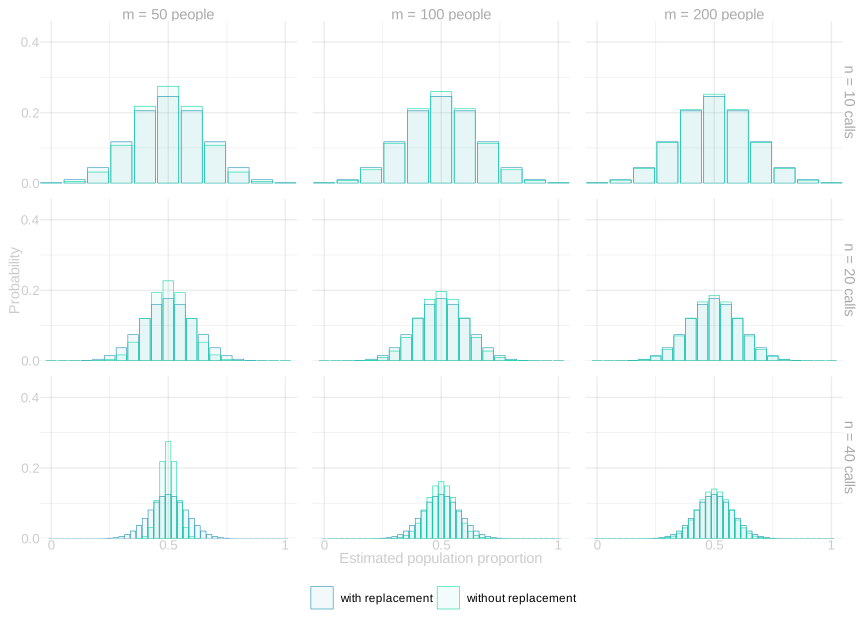
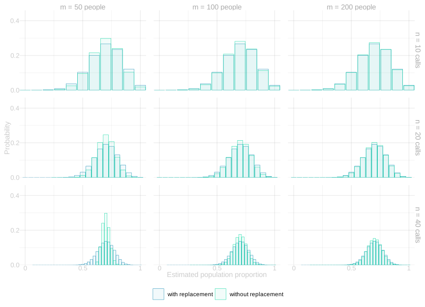
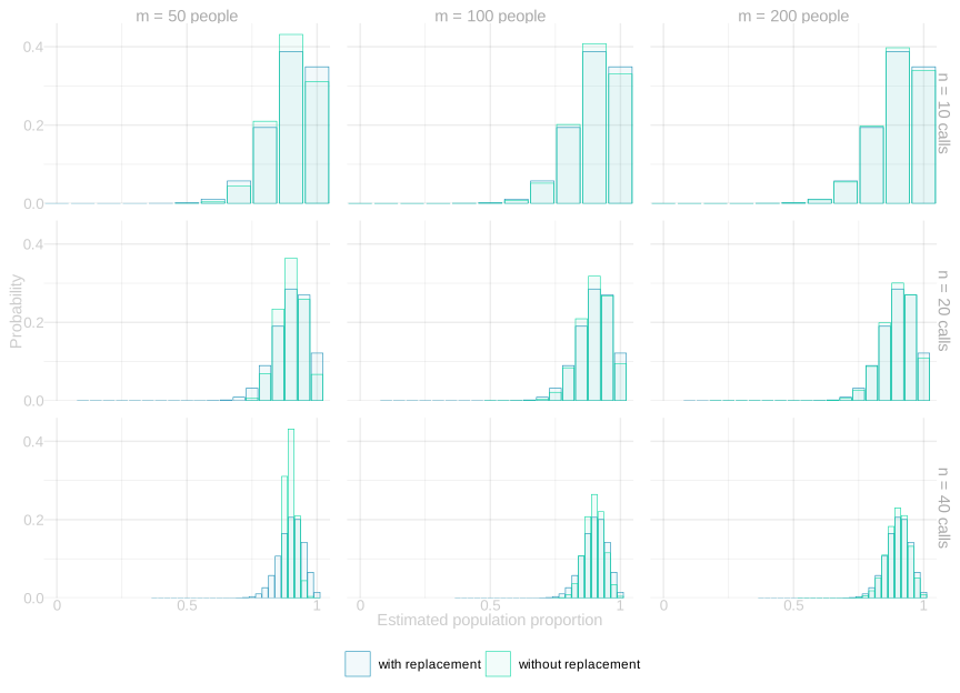
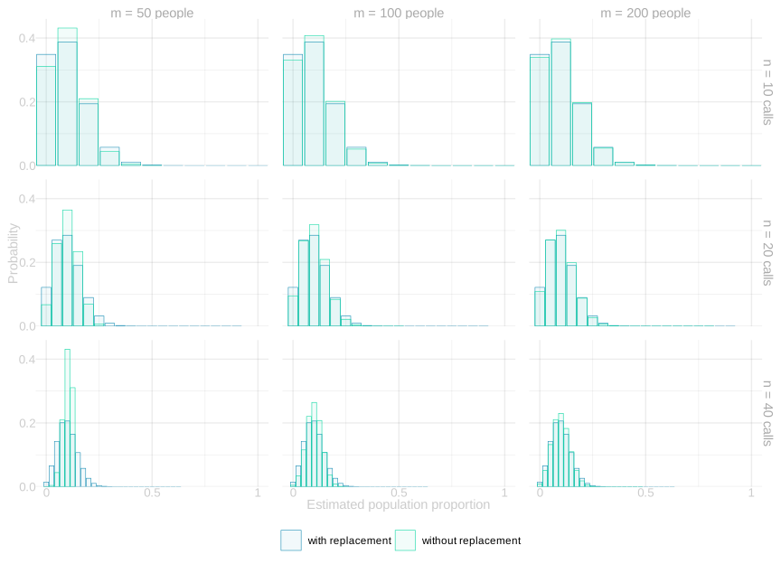
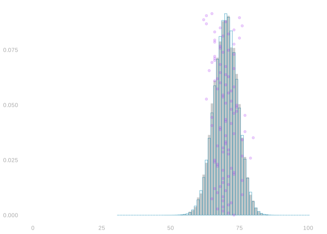
Each panel shows the distribution of the estimated population proportion. Rows change the number of calls \(n\); columns change the population size \(m\). The diagonal keeps \(n/m=1/5\). Use the tabs to change the population proportion \(\theta_1\).

1. Across a row: keep the number of calls fixed. What changes as the population grows? What stays the same?
2. Down the diagonal: increase the number of calls and the population size together. What changes when the fraction sampled stays the same?
3. Between tabs: what changes as the population proportion moves away from one half? How do the last two tabs compare?

Even: \(\theta_1=0.5\)

Figure 11.1

Mid: \(\theta_1=0.7\)

Figure 11.2

Extreme-ish: \(\theta_1=0.9\)

Figure 11.3

Flipped: \(\theta_1=0.1\)

Figure 11.4

The Hypergeometric looks a lot like the Binomial when \(n\) is small relative to \(m\). That’s because sampling without replacement is almost like sampling with replacement when you’re unlikely to pick the same person twice anyway. When \(n\) is a meaningful fraction of \(m\), the Hypergeometric is narrower—you get better precision by not wasting calls on people you’ve already talked to.

If you called everybody you’d know \(\theta_1\) exactly, and there’d be nothing left to be uncertain about.

Using R

The dhyper function gives us the probability: dhyper(s, m1, m0, n) is \(P(\sum_{i=1}^n Y_i = s)\) when we sample \(n\) times without replacement from a population with \(m_1\) ones and \(m_0\) zeros. The rhyper function draws samples: rhyper(10000, m1, m0, n) gives us 10,000.

theta_1 = .7
m = 1000
m1 = m * theta_1
m0 = m * (1-theta_1)
n = 100

p = dhyper(0:n, m1, m0, n)
S = rhyper(10000, m1, m0, n)

ggplot() + geom_col(aes(x=0:n, y=p), fill=pollc, color=pollc, alpha=.05, linewidth=.2) +
           geom_bar(aes(x=S, y=after_stat(prop)), alpha=.3) +
           geom_point(aes(x=S[1:100], y=max(p)*seq(0,1,length.out=100)), 
                      color='purple', alpha=.2)