24  Practice Midterm 1

QTM 285-1

\[ \DeclareMathOperator{\E}{E} \DeclareMathOperator{\Var}{V} \DeclareMathOperator{\hVar}{\widehat{V}} \DeclareMathOperator{\bias}{bias} \DeclareMathOperator*{argmin}{argmin} \newcommand{\model}{\mathcal{M}} \]

Problem 1

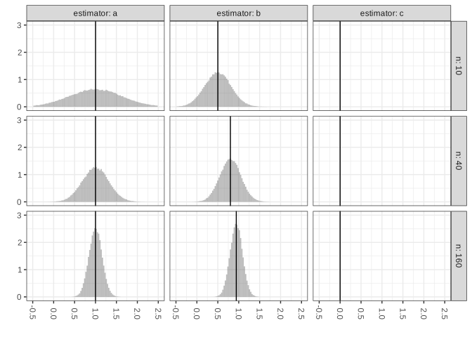
Suppose we’ve drawn a sample \(Y_1 \ldots Y_n\) with replacement from a population \(y_1 \ldots y_m\) with mean \(\theta=\frac{1}{m}\sum_{j=1}^m y_j\). The plot above shows the sampling distributions of these three estimators of \(\theta\). \[ \begin{aligned} \hat \theta_1 &= 0 \\ \hat \theta_2 &= \frac{1}{n}\sum_{i=1}^n Y_i \\ \hat \theta_3 &= \frac{1}{n+10}\sum_{i=1}^n Y_i \end{aligned} \]

ExercisePart A

Match each estimator to the plot of its sampling distribution, e.g. \(\hat\theta_1: a\), \(\hat\theta_2: b\), etc. Of the estimators \(\hat\theta_1\), \(\hat\theta_2\), and \(\hat\theta_3\), which do you know to be consistent? Which could possibly be consistent?

NoteCorrection

The x-axis ticks were mislabeled in the version of this document posted earlier. They were off by 1, so ‘estimator a’ was centered at 0, etc. This has been fixed. I apologize for any confusion this caused.

SolutionSolution

\(\hat\theta_1\) is \(c\), \(\hat\theta_2\) is \(a\), and \(\hat\theta_3\) is \(b\). I know \(\hat\theta_2\) and \(\hat\theta_3\) are consistent, whereas \(\hat\theta_1\) could be consistent but I don’t know that.

Explanation. It’s easy to identify the sampling distribution of \(\hat\theta_1\), as it has no spread at all: it’s always \(0\). And we can differentiate between the sampling distributions of \(\hat\theta_2\) and \(\hat\theta_3\) by observing that \(\hat\theta_2\) (the sample mean) is unbiased, so it must be the one whose center doesn’t change as \(n\) does.

I know \(\hat\theta_2\) and \(\hat\theta_3\) are consistent, as their standard deviations both go to zero as \(n\) goes to infinity and the bias of \(\theta_2\) is zero and that of \(\theta_3\) is \(10\theta/(n+10)\) which goes to zero as \(n\) goes to infinity. I don’t know that \(\hat\theta_1\) is, since its bias is \(-\theta\) no matter what \(n\) is.

But — if you disconnect this part from the sampling distributions I’ve drawn — \(\hat\theta_1\) could be consistent, since its standard deviation does go to zero as \(n\) goes to infinity (it’s zero for all \(n\)) and its bias would be zero if \(\theta\) were \(0\). I wouldn’t take points off for saying it couldn’t be for two reasons. First, I did draw the sampling distributions for you, and what I’ve drawn is inconsistent with \(\theta\) being 0. Second, it’s so rare that anything is ever exactly zero that I wouldn’t fault you for answering the question as if it outright never happened. But that idea—that \(\hat\theta_1\) would be consistent if \(\theta\) were \(0\)—was what I was trying to get at with this could question.

ExercisePart B

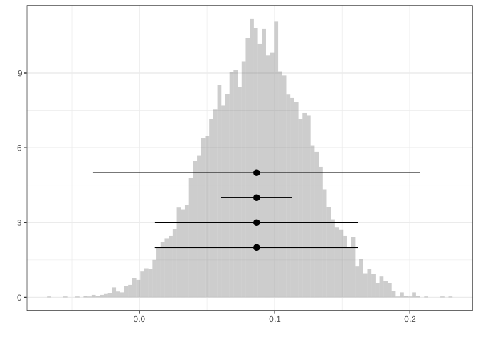
In the plot below, I’ve shown a bootstrap estimate of the sampling distribution of an estimator \(\hat\theta\). Suppose it’s a good estimate, so you can get away with thinking of it as the estimator’s actual sampling distribution. On top of it, I’ve drawn four interval estimators.

• Which are calibrated to have at least 95% coverage? Put a check next to those.
• Which are calibrated to have almost exactly 95% coverage? Circle your check for those.

NoteA Clarification.

If I ask a problem like this on an exam, I’ll make it clear that ‘at least but not exactly 95% coverage’ means substantially more than 95% coverage. Maybe I’ll give you a list of choices for each interval, e.g. 1%, 5%, 50%, 95%, 99% that are spread out enough that familiarity with the illustrations we use often in class will make it clear which is which.

SolutionSolution

From the top, the first, third, and fourth have 95% coverage—the widest 3. The third and fourth have almost exactly 95% coverage.

Explanation. All 3 are wide enough to span at least 95% of draws from (i.e. probability mass of the) sampling distribution. The third and fourth, which are roughly the same, have almost exactly 95% coverage. The first is too wide for that—it spans almost all draws from the sampling distribution.

Problem 2

The miracle of random sampling is that we’re able to estimate the mean of a population with a very small sample from that population. But for that to work, our observations have to be independent—or close to it. If we observe the incomes \(Y_1 \ldots Y_n\) of \(n\) people drawn with replacement from a population with mean income \(\mu\) and income standard deviation \(\sigma\), the variance of the sample mean \(Y_1 \ldots Y_n\) will be \(\sigma^2/n\). Below, I’ve shown the calculation.

\[ \begin{aligned} \Var\sb*{\frac1n\sum_{i=1}^n Y_i} &= \E\sb*{ \cb*{ \frac{1}{n}\sum_i Y_i - \E \p*{ \frac{1}{n}\sum_i Y_i } }^2 } && \\ &= \E\sb*{ \cb*{ \frac{1}{n}\sum_i (Y_i - \E Y_i) }^2 } && \\ &= \E\sb*{ \cb*{ \frac{1}{n}\sum_i Z_i }^2 } && \text{for} \ \ Z_i = Y_i - \E Y_i \\ &= \E\sb*{ \frac{1}{n^2}\sum_i \sum_j Z_i Z_j } && \\ &= \frac{1}{n^2} \sum_i \sum_j \E Z_i Z_j && \\ &= \frac{1}{n^2} \sum_i \sum_j \begin{cases} \sigma^2 & \text{ when } j=i \\ 0 & \text{ otherwise } \end{cases} \\ &= \frac{1}{n^2} \sum_i \sigma^2 = \frac{1}{n^2} \times n \times \sigma^2 = \frac{\sigma^2}{n} \end{aligned} \]

Now suppose that you’ve been lazy, and instead of calling \(n\) different people, you’ve just called one and reported their income \(n\) times. That is, you’ve got ‘a sample of size n’, \(\tilde Y_1 \ldots \tilde Y_n\), with \(\tilde Y_1=Y_1, \tilde Y_2 = Y_1, \tilde Y_3 = Y_1, \ldots\). What is the variance of the mean of this ‘sample’, \(\frac1n\sum_{i=1}^n \tilde Y_i\)? And if it’s not \(\sigma^2/n\) like we got for the mean of \(Y_1 \ldots Y_n\), explain—with reference to the calculation above—why it is not. If there’s a line or lines where something different happens, say which; say what happens instead; and explain why.

SolutionSolution

The variance of this ‘sample mean’ is \(\sigma^2\). The problem is in the second to last line. Note that if we replace each instance of \(Y_i\) with \(\tilde Y_i=Y_1\), then \(Z_i=Y_1 - \E Y_1\) for all \(i\) and \(Z_iZ_j=(Y_1-\E Y_1)^2\) for all \(i\) and \(j\). This means that \(\E Z_i Z_j=\sigma^2\) always instead of only when \(i=j\) and, as a result, \(\frac{1}{n^2}\sum_i\sum_j \E Z_i Z_j\) is an average of \(n^2\) copies of \(\sigma^2\) — one for each pair \((i,j)\).

Problem 3: Interval Calibration

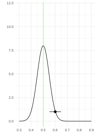
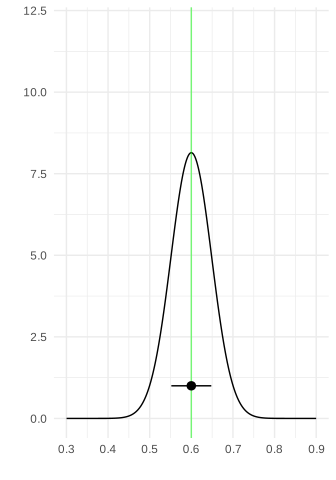
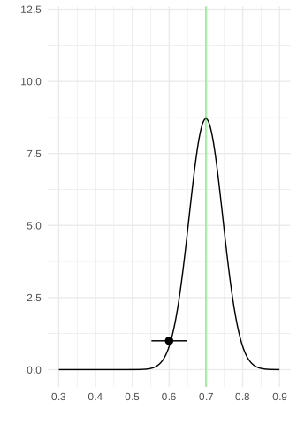
Suppose we’re estimating the proportion \(\theta\) of voters in a population who support a policy, using a sample of size \(n=100\) drawn with replacement. Below are three sampling distributions corresponding to three different values of \(\theta\): 0.5, 0.6, and 0.7. On each, I’ve drawn a 95% confidence interval centered at 0.6.

θ = 0.5

θ = 0.6

θ = 0.7

The green vertical line marks the true value of \(\theta\) in each case.

ExercisePart A

For which of these three values of \(\theta\) does the interval contain the true value? Looking at the sampling distributions, roughly what fraction of intervals constructed this way (centered at \(\hat\theta\) with the same width) would contain \(\theta\) in each case?

SolutionSolution

The interval contains \(\theta\) when \(\theta = 0.6\) (the center plot) and when \(\theta = 0.7\) (the right plot). It does not contain \(\theta\) when \(\theta = 0.5\) (the left plot).

Looking at the sampling distributions:

• When \(\theta = 0.5\): Very few intervals would cover. The sampling distribution is centered at 0.5, but the intervals are centered at whatever \(\hat\theta\) we get. Since \(\hat\theta\) would typically be near 0.5, the intervals would usually be centered near 0.5, and they’d cover \(\theta = 0.5\) about 95% of the time.
• When \(\theta = 0.6\): About 95% of intervals would cover since the interval width was calibrated for this case.
• When \(\theta = 0.7\): About 95% would cover. The sampling distribution is shifted right, but so would our estimates and thus our interval centers.

The key insight is that coverage depends on where \(\hat\theta\) falls relative to \(\theta\), not on where we’ve drawn a single fixed interval.

ExercisePart B

If you wanted to have 95% coverage no matter which of these three \(\theta\) values was true, would you need to make your interval wider, narrower, or keep it the same? Explain briefly.

SolutionSolution

Keep it the same width (or very nearly).

The width of a 95% confidence interval for a proportion is approximately \(1.96\sqrt{\theta(1-\theta)/n}\). This width is largest when \(\theta = 0.5\) and decreases as \(\theta\) moves toward 0 or 1. So the interval calibrated for \(\theta = 0.6\) has width \(1.96\sqrt{0.24/n}\), while the “correct” width for \(\theta = 0.5\) would be \(1.96\sqrt{0.25/n}\) and for \(\theta = 0.7\) would be \(1.96\sqrt{0.21/n}\).

Since \(\sqrt{0.24} \approx 0.49\) is between \(\sqrt{0.25} = 0.5\) and \(\sqrt{0.21} \approx 0.46\), the intervals we’ve drawn are slightly too narrow for \(\theta = 0.5\) and slightly too wide for \(\theta = 0.7\), but the differences are small. In practice, since we don’t know \(\theta\), we estimate the width using \(\hat\theta\), and this gives us close to 95% coverage across a wide range of true \(\theta\) values.

ExercisePart C

Suppose you wanted to achieve 99% coverage instead of 95%. By what factor would you need to multiply the interval width?

Hint: For a normal distribution, 95% of the probability is within \(\pm 1.96\) standard deviations of the mean, and 99% is within \(\pm 2.58\) standard deviations.

SolutionSolution

You would multiply the width by \(2.58/1.96 \approx 1.32\).

The 95% interval has width \(2 \times 1.96 \times \sigma\) and the 99% interval has width \(2 \times 2.58 \times \sigma\), so the ratio is \(2.58/1.96 \approx 1.32\). The 99% interval is about 32% wider than the 95% interval.

Problem 4

In the block of R code below, I’ve implemented the estimators \(\hat\theta_2\) and \(\hat\theta_3\) from Problem 1.

theta.hat.2 = function(Y) { mean(Y) }
theta.hat.3 = function(Y) { sum(Y)/(length(Y)+10) }

And here is code that does a thing.

do.thing = function(estimator) {
  1:10000 |> map_vec(function(.) {
    I = sample(1:n, size=n, replace=TRUE)
    Ystar = Y[I]
    estimator(Ystar)
  }) 
}

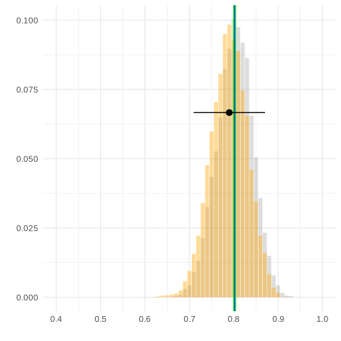
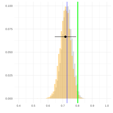
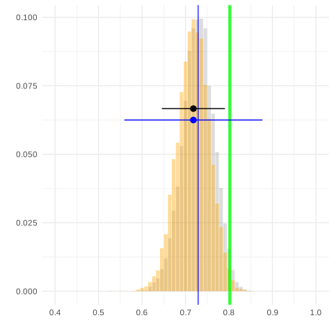
Below, I’ve plotted the sampling distributions of \(\hat\theta_2\) (left) and \(\hat\theta_3\) (right) in gray with their means indicated by blue vertical lines, a histogram of the result of calling do.thing(theta.hat.2) (left) and do.thing(theta.hat.3) (right) in orange, a green vertical line indicating the value of \(\theta\), and interval estimates of the form \(\hat\theta_2 \pm 1.96\hat\sigma_2\) (left) and \(\hat\theta_3 \pm 1.96\hat\sigma_3\) (right) where \(\hat\sigma_2\) and \(\hat\sigma_3\) are the results of calling sd(do.thing(theta.hat.2)) and sd(do.thing(theta.hat.3)) respectively.

ExercisePart A

If we take this approach to calibrating an interval estimator centered on \(\hat\theta_2\), what is the coverage probability of these intervals: roughly 95%, roughly 50%, or roughly 5%? What about the interval estimators centered on \(\hat\theta_3\)?

SolutionSolution

95% for \(\hat\theta_2\) and 50% for \(\hat\theta_3\).

Explanation. The ‘thing’ do.thing does is draw 10,000 samples from the bootstrap sampling distribution of our estimator, so these are the intervals \(\hat\theta \pm 1.96\hat\sigma\) where \(\hat\sigma\) is the standard deviation of the estimator’s bootstrap sampling distributions standard deviation. But we don’t need to know that to answer this question. All we need to know is that, whatever it does, we get histograms with the same widths as our estimators’ actual sampling distributions. That gives us 95% coverage for the unbiased estimator \(\hat\theta_2\), but only about 50% coverage for the estimator \(\hat\theta_3\), which has bias roughly equal to this interval’s width. Why 50%? Because when bias and interval width are equal, we get an interval that covers when our point estimate is on the right half of its sampling distribution and one that doesn’t when it’s on the left half.

ExercisePart B

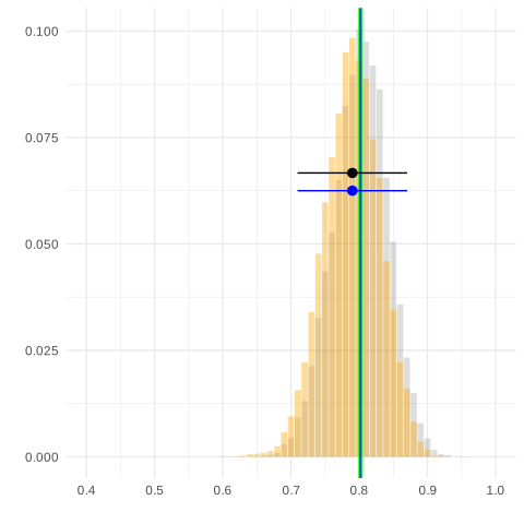
Below, I’ve added another interval estimate to each plot. A blue one. These are \(\hat\theta_2 \pm 1.96 \hat\sigma_2\) and \(\hat\theta_3 \pm 1.96 \hat\sigma_3\) where, letting \(\hat\theta_2^{(1)} \ldots \hat\theta_2^{(10,000)}\) be the elements of do.thing(theta.hat.2) and \(\hat\theta_3^{(1)} \ldots \hat\theta_3^{(10,000)}\) be the elements of do.thing(theta.hat.3), \[ \begin{aligned} \hat\sigma_2^2 &= \frac{1}{10,000}\sum_{r=1}^{10,000} (\hat\theta_2^{(r)} - \bar Y)^2 \\ \hat\sigma_3^2 &= \frac{1}{10,000}\sum_{r=1}^{10,000} (\hat\theta_3^{(r)} - \bar Y)^2. \end{aligned} \]

Explain why the blue interval on the left looks about the same as the black one but the one on the right is wider. Why might you want to use these blue intervals instead of the black ones?

NoteExtra Credit Problems.

This one was meant to be a little unfamiliar—something you couldn’t do on autopilot even if you had perfect recall of the lectures and homeworks. I will put something a bit like this on the exam, but it’ll be an extra credit problem and clearly identified as an extra credit problem. If want to prepare for it, you might want to think a little bit more about \(\hat\sigma_2\) and its relationship to the usual estimate of the standard deviation of the sample mean \(\bar Y\), \(\hat\sigma = \sqrt{\frac{1}{n}\sum_{i=1}^n (Y_i - \bar Y)^2 / n}\).

SolutionSolution

What we’ve done is made \(\hat\sigma\) the root-mean-squared distance of a draw \(\hat\theta^\star\) from our estimator’s bootstrap sampling distribution from the sample’s mean \(\bar Y\) instead of from the bootstrap sampling distribution’s mean. When we’re using the estimator \(\hat\theta_2\), \(\bar Y\) is the bootstrap sampling distribution’s mean, so nothing changes. When we’re using the estimator \(\hat\theta_2\), it’s not—our draws \(\hat\theta^\star\) tend to be lower—so the root-mean-squared distance to \(\bar Y\) is bigger than the standard deviation of \(\hat\theta_2\). We might want to use these because, when we have a biased estimator, they get wider to account for the bias, which improves coverage.

Detail I wouldn’t expect you to provide. In fact, it gets the right amount wider. Think of a point estimate at the left edge of the middle 95% of the sampling distribution of \(\hat\theta_3\)—about where the black interval ends. If you calibrated an interval estimate around it ‘the blue way’, it’d just touch the estimation target. You can see why by thinking about the analogy that motivates the bootstrap.

About the Bootstrap. When we use the bootstrap, we’re thinking of the relationship between a bootstrap sample and the sample as analogous to the relationship between the sample and population. So what we’re really doing here is calculating the root-mean-squared difference between a bootstrap version of our estimator, \(\hat\theta^\star\), to a bootstrap version of our estimation target, \(\theta^\star=\bar Y\)—that’s the mean of the ‘population’ that our bootstrap sample is drawn from. When \(\hat\theta^\star\) an an unbiased estimator of \(\theta^\star\), this is just its standard deviation. But when \(\hat\theta^*\) is a biased estimator of \(\theta^\star\), it’s a bootstrap version of root-mean-squared-error. \[ \text{bootstrap rmse} = \sqrt{\text{bootstrap bias}^2 + \text{bootstrap sd}^2}. \] Often, the bootstrap analogy works and the bootstrap bias and bootstrap sd are about the same as the actual bias and actual sd. This mean we’ll get 95% coverage from our biased estimator, as we’re inflating the width of our intervals just enough that that happens. That is not, however, necessarily the best way to take advantage of our ability to use the bootstrap to anticipate our estimator’s bias. Instead of using it to inflate the width of our intervals, we can use it to correct the bias of our estimator so we don’t have to inflate them. More on this later in the semester.