8  Sampling with Replacement and the Binomial Distribution

Sampling with Replacement

To calibrate our intervals, we need to understand the sampling distribution of our estimator. That means doing some probability calculations. The machinery isn’t complicated—we’ll count equally likely configurations and add up probabilities—but it gets notationally heavy when we apply it to the polling problem. So let’s warm up on something simpler first.

You’ve done this already, near enough. In the first homework you took six die sides, added a column for whether each was 3 or more—free, because the roll determines it—and added up the rows that agreed. What follows isn’t quite that. It’s a version of it, with people instead of sides and their answers instead of an indicator.

Finding the Distribution of \(Y_1\) in a Small Population

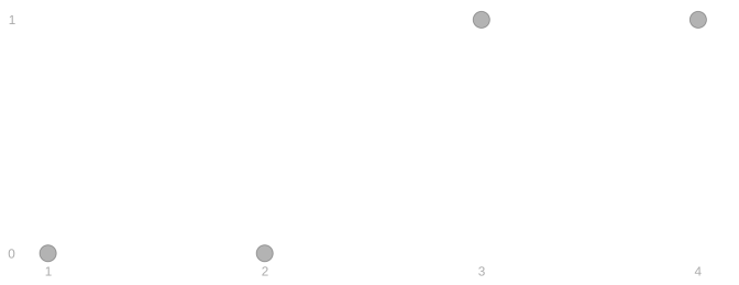
Let’s start with the distribution of \(Y_1\), the response to one call, when we sample with replacement. And to keep things concrete, let’s suppose we’re polling a population of size \(m=4\). We’re rolling a 4-sided die.

NoteIf you have a deck of cards

You can put this on the table instead of reading it.

Lay your population out: a red card for each voter who’ll vote, a black one for each who won’t. Four cards here, two of each. Roll a die to pick who you call — or just imagine rolling it — and turn that card over.

Red or black is what you heard. There are two reds, so there are two rolls that get you a Yes, and that is the whole of the \(2/4\).

The Population

\(j\) name \(y_j\)
\(1\) Rush \(0\)
\(2\) Mitt \(0\)
\(3\) Al \(1\)
\(4\) Newt \(1\)

The Joint

\(p\) \(J_1\) \(Y_1\)
\(\color{#EF476F}\frac14\) \(1\) \(\color{#EF476F}0\)
\(\color{#EF476F}\frac14\) \(2\) \(\color{#EF476F}0\)
\(\color{\) \(3\) \(\color{\)
\(\color{\) \(4\) \(\color{\)

The Marginal

\(p\) \(Y_1\)
\(\color{#EF476F}\frac24\) \(\color{#EF476F}0\)
\(\color{\) \(\color{\)

We have two Nos (0s) and two Yeses (1s). The ‘Yes’ frequency in the population is \(\theta_1 = 2/4\). Here’s how we find the distribution of \(Y_1\).

  1. We write the probability distribution of our die roll in a table. It has two columns: one for the roll \(J_1\) and another for its probability \(p\). It has \(m=4\) rows, one for each possible outcome of the roll. Each roll is equally likely, so the probability in each row is \(1/4\).

  2. We add a column for the response to our call, \(Y_1\). Adding this column is ‘free’—it doesn’t change the row’s probability—because what we hear is determined by the roll. E.g. if we roll a 1, we’re going to hear Rush say ‘No’. So the probability we roll a 1 and hear a ‘No’ is the same as the probability we roll a 1.

  3. We marginalize over rolls to find the distribution of our call’s outcome. We can color each row according to the call’s outcome \(Y_1\), then sum the probabilities in each color. The probability of hearing ‘No’ is the probability that we roll a 1 or 2: \(1/4+1/4 = 2/4\). The probability of hearing ‘Yes’ is the probability that we roll a 3 or 4: \(2/4\). These probabilities match the frequencies of ‘Yes’ and ‘No’ in our population.

Index Sets and Summands

A sum has two parts. There’s the set of things you walk over, and there’s what you write down for each one.

\[ \sum_{j \,\in\, 1 \ldots 4} \frac{1}{4} \qquad\longrightarrow\qquad \sum_{j \,\in\, \{\,j \,:\, y_j = 0\,\}} \frac{1}{4} \]

Both have the same summand, \(1/4\). What changed is the index set: on the left it’s everybody, \(1 \ldots 4\); on the right it’s the ones who said No, which here is \(\{1, 2\}\).1

So the right-hand sum is \(1/4 + 1/4\), and the marginal we just wrote down is that sum.

The size of an index set is worth a name of its own, because we’ll be counting them from here on.

\[ m_y = \sum_{j \,\in\, \{\,j \,:\, y_j = y\,\}} 1 \]

That’s the number of voters who’d say \(y\). Here \(m_0 = 2\) and \(m_1 = 2\), and \(m_0 + m_1 = m = 4\).

Generalizing to Larger Populations

Nothing we just did used the fact that there were four voters. So let’s do it again without a number in it, for a binary population \(y_1 \ldots y_m\) of any size \(m\). To ground us while we do it, we’ll think about our population of \(m=7.23M\) registered voters in Georgia. But we’ll handle the general case. Plugging in 7.23M ones and zeros wouldn’t exactly make things easier.

Finding the Distribution of \(Y_1\) in a Large Population

The Population

\(j\) \(y_j\)
\(1\) 1
\(2\) 1
\(3\) 1
\(4\) 0
\(m\) 1

The Joint

\(p\) \(J_1\) \(Y_1\)
\(1/m\) \(1\) \(1\)
\(1/m\) \(2\) \(1\)
\(1/m\) \(3\) \(1\)
\(1/m\) \(4\) \(0\)
\(1/m\) \(m\) \(1\)

The Marginal

\(p\) \(Y_1\)
\(\underset{\color{gray}\approx 0.30}{\sum\limits_{j:y_j=0} \frac{1}{m}}\) \(0\)
\(\underset{\color{gray}\approx 0.70}{\sum\limits_{j:y_j=1} \frac{1}{m}}\) \(1\)
  1. We start by writing the probability distribution of our dice rolls. The person we call, \(J_1\), is equally likely to be anyone in the population of \(m \approx 7.23M\) people. It takes on each value \(1 \ldots m\) with probability \(1/m\).

  2. We add a column for the response to our call, \(Y_1\). This is ‘for free’. The roll determines what we hear, so the probabilities don’t change. Still \(1/m\).

  3. And we marginalize to find the distribution of \(Y_1\). We sum the probabilities in rows where \(Y_1=0\) and \(Y_1=1\). What we saw in our small population does generalize. The probability of hearing a response \(y \in \{0,1\}\) is the frequency of that response in the population. We’ll call these frequencies \(\theta_0\) and \(\theta_1\). This is a little redundant because \(\theta_0 = 1 - \theta_1\). Our estimation target is just the ‘Yes’ frequency \(\theta_1\). Some people call it the success rate.

To find the distribution of a sum of \(Y_1+Y_2\), we can follow the same steps. There’s a bit more to it, so we’ll break down the marginalization step to make it a little more tractable.

Two Calls to A Small Population

\(j\) name \(y_j\)
\(1\) Rush \(0\)
\(2\) Mitt \(0\)
\(3\) Al \(1\)
\(4\) Newt \(1\)

Four-person binary population: outcomes zero at indices one and two, one at indices three and four.

Two calls now. We make a table for the joint distribution of two rolls, add the response columns for free as before, and marginalize twice — once to get the responses, once to get their sum.

There are \(4 \times 4 = 16\) equally likely pairs of rolls, each with probability \(1/16\). Few enough to write down, so let’s write them all down. The response columns come along for free, same as before, and so does their sum.

NoteIf you have a deck of cards

Deal the whole thing out. Turn up two cards, left one first, write down what you heard, put them back, and go again until you have all sixteen pairs.

Keep the ones that sound the same together and you’ll finish with four piles of four, which is the table below in the order it’s written.

The Joint

\(p\) \(J_1\) \(J_2\) \(Y_1\) \(Y_2\) \(Y_1 + Y_2\)
\(\color{#EF476F}\frac{1}{16}\) \(1\) \(1\) \(0\) \(0\) \(0\)
\(\color{#EF476F}\frac{1}{16}\) \(1\) \(2\) \(0\) \(0\) \(0\)
\(\color{#EF476F}\frac{1}{16}\) \(2\) \(1\) \(0\) \(0\) \(0\)
\(\color{#EF476F}\frac{1}{16}\) \(2\) \(2\) \(0\) \(0\) \(0\)
\(\color{\) \(1\) \(3\) \(0\) \(1\) \(1\)
\(\color{\) \(1\) \(4\) \(0\) \(1\) \(1\)
\(\color{\) \(2\) \(3\) \(0\) \(1\) \(1\)
\(\color{\) \(2\) \(4\) \(0\) \(1\) \(1\)
\(\color{\) \(3\) \(1\) \(1\) \(0\) \(1\)
\(\color{\) \(3\) \(2\) \(1\) \(0\) \(1\)
\(\color{\) \(4\) \(1\) \(1\) \(0\) \(1\)
\(\color{\) \(4\) \(2\) \(1\) \(0\) \(1\)
\(\color{\) \(3\) \(3\) \(1\) \(1\) \(2\)
\(\color{\) \(3\) \(4\) \(1\) \(1\) \(2\)
\(\color{\) \(4\) \(3\) \(1\) \(1\) \(2\)
\(\color{\) \(4\) \(4\) \(1\) \(1\) \(2\)

They’re in an order that makes them easy to count: the rows where you’d hear No-No, then No-Yes, then Yes-No, then Yes-Yes. Four rows in each group.

Add them up by colour and you have the distribution of \(Y_1+Y_2\): \(4/16\) for a sum of \(0\), \(8/16\) for a sum of \(1\) because two of the groups give that sum, and \(4/16\) for a sum of \(2\).

Two Calls to A Large Population

Ten Voters

ExerciseTwo Calls to Ten Voters

Ten voters now, \(m_1\) of whom will vote and \(m_0\) of whom won’t. We make the same two calls.

Find the distribution of \(Y_1 + Y_2\).

There are a hundred pairs of rolls this time. You can write all hundred out the way we just did, and it will work, but see whether you can get the answer without writing them out.

NoteIf you have a deck of cards

Deal yourself ten, however many red you like, and that’s your population — \(m_1\) reds and \(m_0\) blacks. Roll a ten-sided die twice, or point at two cards without looking, and that’s your pair of calls.

Writing out a hundred rows works and it’s horrible. What makes it horrible is that you’re doing the whole thing in one go, so let’s do it in two stages instead.

The first stage collapses the rolls into what you’d hear. Every pair of rolls that sounds the same becomes one row, and the probability of that row is the probability of the whole group. That’s partial marginalization — partial because you still have \(Y_1\) and \(Y_2\) in front of you, not their sum. The second stage collapses those into the sum, adding the rows that agree. That’s full marginalization.

Here’s the four voters again, done in those two stages.

Partially Marginalized

\(p\) \(Y_1\) \(Y_2\) \(Y_1 + Y_2\)
\(\color{#EF476F}\frac{4}{16}\) \(0\) \(0\) \(0\)
\(\color{\) \(0\) \(1\) \(1\)
\(\color{\) \(1\) \(0\) \(1\)
\(\color{\) \(1\) \(1\) \(2\)

Fully Marginalized

\(p\) \(Y_1 + Y_2\)
\(\color{#EF476F}\frac{4}{16}\) \(0\)
\(\color{\) \(1\)
\(\color{\) \(2\)

The \(8\) is \(2 \times 4\), because ‘No,Yes’ and ‘Yes,No’ are two different things to hear that happen to give the same sum.

And the four rows of the first table don’t need the sixteen underneath them either. Take ‘Yes,No’. Al and Newt are the two who’d say Yes, so two rolls give you the Yes on the first call. Rush and Mitt are the two who’d say No, so whichever of those you got, two rolls give you the No on the second. Two choices and then two choices, \(2 \times 2 = 4\), and you never wrote a pair down.

NoteIf you have a deck of cards

Put down a red then a black, a Yes then a No. Swap that red for the other red: you called somebody else and heard the same thing. Swap the black for the other black and the same happens again.

Two reds to choose from, two blacks, and you can lay all four of those pairs out at once and look at them.

Now you do this one.

Partially Marginalized

\(p\) \(Y_1\) \(Y_2\) \(Y_1 + Y_2\)
  \(0\) \(0\) \(0\)
  \(0\) \(1\) \(1\)
  \(1\) \(0\) \(1\)
  \(1\) \(1\) \(2\)

Then collapse it by the last column.

Take ‘Yes,No’. There are \(m_1\) rolls that give you the Yes and \(m_0\) that give you the No, so \(m_1 m_0\) pairs sound like that — out of \(10 \times 10 = 100\) pairs in all.

Partially Marginalized

\(p\) \(Y_1\) \(Y_2\) \(Y_1 + Y_2\)
\(\color{#EF476F}\frac{m_0 m_0}{100}\) \(0\) \(0\) \(0\)
\(\color{\) \(0\) \(1\) \(1\)
\(\color{\) \(1\) \(0\) \(1\)
\(\color{\) \(1\) \(1\) \(2\)

Fully Marginalized

\(p\) \(Y_1 + Y_2\)
\(\color{#EF476F}\frac{m_0 m_0}{100}\) \(0\)
\(\color{\) \(1\)
\(\color{\) \(2\)

Only the counts moved. Four voters, two of each, gave \(2 \times 2\) over \(16\). Ten gives \(m_1 m_0\) over \(100\).

Checking Your Answer

Put your own numbers in and run it. It works for any of the exercises in this chapter — change n to three or to six hundred and it still answers.

Any Number of Voters

ExerciseGeneralize It

Now \(m\) voters. \(m_1\) of them will vote, \(m_0\) won’t. Same two calls.

Don’t do it again from scratch. Take the answer you just wrote for the ten and cross out every number that came from there being ten of them and write the general thing in its place.

Partially Marginalized

\(p\) \(Y_1\) \(Y_2\) \(Y_1 + Y_2\)
\(\color{#EF476F}\frac{m_0 m_0}{m^2}\) \(0\) \(0\) \(0\)
\(\color{\) \(0\) \(1\) \(1\)
\(\color{\) \(1\) \(0\) \(1\)
\(\color{\) \(1\) \(1\) \(2\)

Fully Marginalized

\(p\) \(Y_1 + Y_2\)
\(\color{#EF476F}\frac{m_0 m_0}{m^2}\) \(0\)
\(\color{\) \(1\)
\(\color{\) \(2\)

Dividing each count by \(m\) as you go, these are products of the frequencies: \(\theta_0\theta_0\), \(\theta_0\theta_1\), \(\theta_1\theta_0\), \(\theta_1\theta_1\).

Three Calls to A Large Population

By now we’ve got our steps down. First partial marginalization, from rolls to responses. Then full marginalization, from responses to their sum.

NoteIf you have a deck of cards

Ten cards, \(m_1\) of which are red and \(m_0\) black. Three calls is three rolls of the die, and the three cards you turn up, left to right, are one row of your table: the colours are what you heard and the position is which call you heard it on.

Two things you can do to a row like that, and they are the two stages.

Understanding partial marginalization. Swap a card for another of the same colour. You called somebody else and you heard the same thing. The row doesn’t move; you’ve found another roll sequence sitting underneath it, and counting those is what the first stage does.

Understanding full marginalization. Move the cards you have into a different order. Now you’ve got a different row — a different thing to hear — with the same number of Yeses in it, so it lands on the same sum. Counting those is what the second stage does.

ExerciseThree Calls

Three calls to the same ten voters. Same question: the distribution of the sum.

Give a row a name. What you hear on three calls is a sequence of three answers \(a_1 a_2 a_3\), each one a \(0\) or a \(1\), and there are eight such sequences.

The probability of hearing \(a_1 a_2 a_3\) is the number of roll sequences that produce it over the number of roll sequences there are, and you count it the way you counted pairs.

\[ p(a_1 a_2 a_3) = \frac{m_{a_1} m_{a_2} m_{a_3}}{10^3} \qqtext{where} m_y = \sum_{j \,\in\, \{\,j \,:\, y_j = y\,\}} 1 \]

Now put the same answers in a different order. Hearing \(1 0 0\), hearing \(0 1 0\) and hearing \(0 0 1\) are three different things, three different rows of your table, and their probabilities are \(m_1 m_0 m_0\), \(m_0 m_1 m_0\) and \(m_0 m_0 m_1\) over \(10^3\). Moving the Yes moves a factor. It does not change the product.

Collapsing by the sum means summing over the sequences that give that sum.

\[ \sum_{\substack{a_1 a_2 a_3 \\ a_1 + a_2 + a_3 \,=\, s}} \frac{m_{a_1} m_{a_2} m_{a_3}}{10^3} \]

The index set is the sequences with \(s\) Yeses. The summand is the same for every one of them, by what you just noticed. And a sum of a constant is that constant times the size of the index set, so the only thing left to find is how big that index set is.

Each of the eight things you could hear has three counts multiplied together underneath it, one per call, for the same reason as before — and \(10 \times 10 \times 10 = 10^3\) roll sequences in all.

Partially Marginalized

\(p\) \(Y_1\) \(Y_2\) \(Y_3\) \(Y_1+Y_2+Y_3\)
\(\color{#EF476F}\frac{m_0^3}{10^3}\) \(0\) \(0\) \(0\) \(0\)
\(\color{\) \(0\) \(0\) \(1\) \(1\)
\(\color{\) \(0\) \(1\) \(0\) \(1\)
\(\color{\) \(0\) \(1\) \(1\) \(2\)
\(\color{\) \(1\) \(0\) \(0\) \(1\)
\(\color{\) \(1\) \(0\) \(1\) \(2\)
\(\color{\) \(1\) \(1\) \(0\) \(2\)
\(\color{#FFD166}\frac{m_1^3}{10^3}\) \(1\) \(1\) \(1\) \(3\)

Fully Marginalized

\(p\) \(Y_1+Y_2+Y_3\)
\(\color{#EF476F}\frac{m_0^3}{10^3}\) \(0\)
\(\color{\) \(1\)
\(\color{\) \(2\)
\(\color{#FFD166}\frac{m_1^3}{10^3}\) \(3\)

The left-hand column of the second table carries the multipliers \(1, 3, 3, 1\).

The counts adapted from two calls exactly as you’d expect: two factors became three. The \(1,3,3,1\) didn’t adapt from anything. With two calls there were two ways to hear one Yes and you could see both at once; with three there are three, and you had to write them out to be sure.

\(n\) Calls to A Large Population

Exercise\(n\) Calls

Two calls gave you four things you could hear. Now make \(n\) calls to the same \(m\) voters.

Work out the distribution of \(Y_1 + \ldots + Y_n\). Use the same approach: partial marginalization first, from rolls to responses, then full marginalization, from responses to their sum.

The first stage is the multiplication you’ve done three times now, run \(n\) times instead of two or three. A row with \(s\) Yeses and \(n-s\) Nos has \(m_1^s m_0^{n-s}\) roll sequences under it, out of \(m^n\).

The second stage is the one that stops you. There are \(2^n\) things you could hear and you are not going to write them down. You don’t need to. Every one of them with \(s\) Yeses carries the same probability, so the only thing the second stage asks of you is how many of them have \(s\) Yeses.

You don’t have to be able to work that number out to finish the calculation. Give it a name and carry it.

Stop half way and fill this in first.

Partially Marginalized

\(p\) \(Y_1\) \(Y_2\) \(\ldots\) \(Y_n\) \(Y_1 + \ldots + Y_n\)
  \(0\) \(0\) \(\ldots\) \(0\) \(0\)
  \(0\) \(0\) \(\ldots\) \(1\) \(1\)
  \(1\) \(1\) \(\ldots\) \(1\) \(n\)

\(2^n\) rows, one per thing you could hear. Then collapse that by the last column.

To find the distribution of a sum \(Y_1 + \ldots + Y_n\), we do the same thing. We start by writing out the joint distribution of \(n\) dice rolls. We’re equally likely to roll any sequence of \(n\) numbers in \(1\ldots m\). And there are \(m^n\) sequences, so the probability is \(1/m^n\) for each sequence. Then we add columns for the corresponding responses ‘for free’. And the sums.

Then we marginalize in two steps.

  1. Sum over roll sequences leading to the same response sequence \(a_1 \ldots a_n\).
  2. Sum over response sequences leading to the same sum \(s=a_1+\ldots+a_n\).

Step 1. Partial Marginalization

Here’s the table we stopped at half way, with the probability column filled in. Every row is a product of \(n\) frequencies, one per call, and which product it is depends only on how many of the calls were Yeses.

Partially Marginalized

\(p\) \(Y_1\) \(Y_2\) \(\ldots\) \(Y_n\) \(Y_1 + \ldots + Y_n\)
\(\color{#EF476F}\theta_0^n\) \(0\) \(0\) \(\ldots\) \(0\) \(0\)
\(\color{\) \(0\) \(0\) \(\ldots\) \(1\) \(1\)
\(\color{\) \(1\) \(1\) \(\ldots\) \(0\) \(n-1\)
\(\color{#FFD166}\theta_1^n\) \(1\) \(1\) \(\ldots\) \(1\) \(n\)

To sum over roll sequences, we sum over one roll after another. This is exactly like what we did for one response. Except over and over. You can think of this sum ‘inside out.’

Suppose we’re calculating the probability of the response sequence \(a_1 \ldots a_n = 0,0,...,0,0\).

  1. We consider any ‘head’ \(j_1\ldots j_{n-1}\) where \(y_{j_1} \ldots y_{j_{n-1}}=0,0,...0\) and think about choosing the last element. No matter what the head is, there are \(m_0\) ways to complete it by choosing \(j_{n}\) with \(y_{j_n}=0\).
  2. We repeat with shortened ‘head’ \(j_1 \ldots j_{n-2}\) to consider the choice of \(j_{n-1}\). We have \(m_0\) choices and our last step tells us that each choice results in \(m_0\) call sequences, so there are \(m_0^2\) sequences with head \(j_1 \ldots j_{n-2}\) ending in \(0,0\).
  3. Repeat \(n-2\) more times.

What we get is pretty similar to the two-response case. The probability of observing the sequence is determined by the frequency of Yeses and Nos in the population. It’s the product of the frequencies of those responses. For ‘Yes,Yes,…,Yes’ it’s \(\theta_1^n\). For ‘No,No,…,No’ it’s \(\theta_0^n\). And if we have \(s\) Yeses and therefore \(n-s\) Nos, it’s \(\theta_1^s\theta_0^{n-s}\).

This is, again, the product of the marginal probabilities of those \(n\) responses.

\[ \begin{aligned} \sum_{\substack{j_1 \ldots j_n \\ y_{j_1} \ldots y_{j_n} = a_1 \ldots a_n}} \frac{1}{m^n} &= \sum_{\substack{j_1 \ldots j_{n-1} \\ y_{j_1} \ldots y_{j_{n-1}} = a_1 \ldots a_{n-1}}} \sum_{\substack{j_n \\ y_n=a_n}} \frac{1}{m^n} \\ &= \sum_{\substack{j_1 \ldots j_{n-1} \\ y_{j_1} \ldots y_{j_{n-1}} = a_1 \ldots a_{n-1}}} \sum_{\substack{j_n \\ y_n=a_n}} m_{a_n} \times \frac{1}{m^n} \\ &= \sum_{\substack{j_1 \ldots j_{n-2} \\ y_{j_1} \ldots y_{j_{n-2}} = a_1 \ldots a_{n-2}}} \sum_{\substack{j_{n-1} \\ y_n=a_{n-1}}} m_{a_n} \times \frac{1}{m^n} \\ &= \sum_{\substack{j_1 \ldots j_{n-2} \\ y_{j_1} \ldots y_{j_{n-2}} = a_1 \ldots a_{n-2}}} \sum_{\substack{j_{n-1} \\ y_n=a_{n-1}}} m_{a_{n-1}} m_{a_n} \times \frac{1}{m^n} \\ &= m_{a_1} \ldots m_{a_{n}} \times \frac{1}{m^n} \qqtext{after repeating $n-2$ more times} \\ &= \theta_{a_1} \ldots \theta_{a_n} \\ &= \prod_{i:a_i=1} \theta_1 \prod_{i:a_i=0} \theta_0 = \theta_1^{s} \theta_0^{n-s} \qfor s = a_1 + \ldots + a_n \end{aligned} \]

Step 2. Full Marginalization

Collapsing that table by its last column, every sum from \(0\) to \(n\) gets one row, and the multiplier on each is the number of response sequences with that many Yeses, written \(\binom{n}{s}\) and spoken ‘\(n\) choose \(s\)’.

Fully Marginalized

\(p\) \(Y_1 + \ldots + Y_n\)
\(\color{#EF476F}\binom{n}{0} \theta_0^n\) \(0\)
\(\color{\) \(1\)
\(\color{\) \(n-1\)
\(\color{#FFD166}\binom{n}{n} \theta_1^n\) \(n\)

The full marginalization step is a bit trickier. But we can take advantage of our partial marginalization. To calculate the probability that the sum takes on the value \(s\), we order our sum of probabilities thoughtfully. We sum over response sequences \(a_1 \ldots a_n\) with \(s\) Yeses and \(n-s\) Nos. And within that, we sum over calls where we’d hear those responses.

The inner sum we’ve done. That was our partial marginalization. And the outer sum boils down to counting the number of sequences with \(s\) Yeses. The probability of all these sequences is the same: \(\theta_1^s\theta_0^{n-s}\). So summing is counting and multiplying. You may have done the counting part in high school in a unit on ‘permutations and combinations’. In any case, that count has a name. It’s spoken ‘\(n\) choose \(s\)’ and written \(\binom{n}{s}\).

\[ \begin{aligned} \sum\limits_{\substack{j_1 \ldots j_n \\ y_{j_1} + \ldots + y_{j_n} = s}} \frac{1}{m^n} &= \sum\limits_{\substack{a_1 \dots a_n \\ a_1 + \ldots + a_n = s}} \ \ \sum_{\substack{j_1 \ldots j_n \\ y_{j_1} \ldots y_{j_n} = a_1 \ldots a_n}} \frac{1}{m^n} \\ & =\sum\limits_{\substack{a_1 \dots a_n \\ a_1 + \ldots + a_n = s}} \theta_1^{s}\theta_0^{n-s} \\ &= \binom{n}{s} \theta_1^{s} \theta_0^{n-s} \qqtext{ where } \binom{n}{s} = \sum\limits_{\substack{a_1 \dots a_n \\ a_1 + \ldots + a_n = s}} 1 \end{aligned} \]

Using R

\[ P\left(\sum_{i=1}^n Y_i = s\right) = \binom{n}{s} \theta_1^{s}\theta_0^{n-s} \ \ \text{ where } \ \ \binom{n}{s} \text{ is the number of binary sequences $a_1 \ldots a_n$ summing to $s$.} \]

We don’t actually have to do all this sequence-summing-to-\(s\) counting ourselves. The choose function in R will do it for us: \(\binom{n}{s}\) is choose(n,s). The dbinom function will give us the whole probability: \(\binom{n}{s}\theta_1^s\theta_0^{n-s}\) is dbinom(s, n, theta_1). And the rbinom function will draw samples from this distribution: rbinom(10000, n, theta_1) gives us 10,000.

theta_1 = .7
n = 625
p = dbinom(0:n, n, theta_1)
S = rbinom(10000, n, theta_1)

ggplot() + geom_area(aes(x=0:n,   y=p), color=pollc, alpha=.2) +
           geom_bar(aes(x=S, y=after_stat(prop)), alpha=.3) +
           geom_point(aes(x=S[1:100],   y=max(p)*seq(0,1,length.out=100)), 
                      color='purple', alpha=.2)
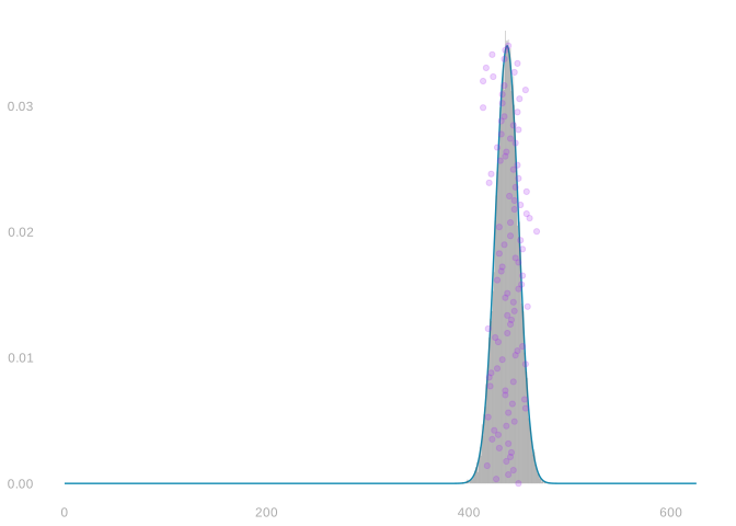
Exact Binomial probability curve for a count with 625 trials and success probability .7, overlaid with a simulated histogram and 100 simulated counts.

The Binomial Distribution

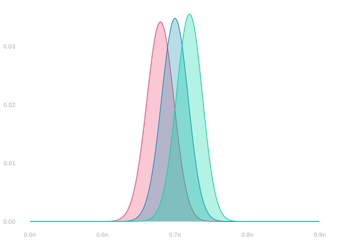
Three overlapping Binomial count distributions for success probabilities .68, .70, and .72; increasing the probability shifts the distribution right.

\[ \begin{aligned} &\overset{\color{gray}=P\left(\frac{1}{n}\sum_{i=1}^n Y_i = \frac{s}{n}\right)}{P\left(\sum_{i=1}^n Y_i = s\right)} = \binom{n}{s} \theta_1^{s}\theta_0^{n-s} \\ &\qfor n =625 \\ &\qand \theta_1 \in \{\textcolor[RGB]{239,71,111}{0.68}, \textcolor[RGB]{17,138,178}{0.7}, \textcolor[RGB]{6,214,160}{0.72} \} \end{aligned} \]

These functions have ‘binom’ in their name because we call this distribution the Binomial distribution. The Binomial distribution on \(n\) trials with success probability \(\theta\) is our name for the distribution of the sum of \(n\) binary random variables with probability \(\theta\) of being \(1\). E.g. the number of heads in \(n\) coin flips is Binomial with \(n\) trials and success probability \(1/2\).

We’ve shown that’s the sampling distribution of the sum of responses, \(Y_1 + \ldots + Y_n\), when we sample with replacement from a population of binary responses \(y_1 \ldots y_m\) in which \(\theta\) is the frequency of ones. We’re interested in the mean of responses, so we divide by \(n\): \(\color{gray} \sum_{i=1}^n Y_i = s \ \text{ when } \ \frac{1}{n}\sum_{i=1}^n Y_i = s/n\).

It’s easy to estimate—and talk about estimating—this sampling distribution. It depends only on one thing we don’t know: the population frequency \(\theta\). And that’s exactly the thing we’re trying to estimate anyway. That’s why we’ve started here—the case of sampling with replacement from a population of binary responses.

Getting the Same Picture by Calling People

We got that curve by counting. You can also get it by calling people. Draw \(n\) callees with replacement, look up what each one says, add them up, and do that ten thousand times.

one.sample.sum = function() sum(y[sample(m, n, replace=TRUE)])
S = replicate(10000, one.sample.sum())

ggplot() + geom_bar(aes(x=S, y=after_stat(prop)), alpha=.3) +
           geom_area(aes(x=0:n, y=dbinom(0:n, n, mean(y))), color=pollc, alpha=.2) +
           coord_cartesian(xlim=c(.6,.8)*n)
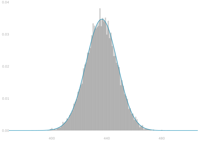
Simulated histogram of the response sum from ten thousand samples of 625 calls, with the exact Binomial curve drawn over it.

The histogram is what happened when we called people; the curve is \(\binom{n}{s}\theta_1^s\theta_0^{n-s}\) with \(\theta_1\) read off the population. Nothing in the code knows about the curve and nothing in the curve knows about the code.


  1. You’ll also see the left-hand one written \(\sum_{j=1}^{4}\). Same meaning—it’s naming the index set by its first and last element instead of writing the set out.↩︎